B-plot writes when the script runsDictionary of Applied Machine Learning · supervised learning
Numerical companion to the entry supervised learning: it recomputes what the entry states and prints one line per check
Numerical companion to the glossary entry 'supervisedlearning'. The GeoSphere Austria weather station Krems (station id 3805) records the minimum and the maximum air temperature of each day; this script downloads the records for 2024 from the GeoSphere data hub (dataset klima-v2-1d) and writes them to supervisedlearning_weather.csv. Each day is a data point. Its feature is the morning minimum temperature, its label the maximum temperature of that day. Both numbers are measured, so every data point of the training set carries its label, which is what makes the setting supervised.
Run it with python3 supervisedlearning.py, from any directory — it writes its output files into the current directory. Requires NumPy and Matplotlib only, and uses fixed seeds, so the printed numbers reproduce exactly. Download supervisedlearning.py · Notebook · Open in Colab
One cell per block of the script: the code, and what that code printed when it last ran here
"""Supervised learning on a year of days at Krems: each day carries a
label, ERM fits a hypothesis to the labeled days, and the same labels
serve a regression and a classification problem.

Purpose
-------
Numerical companion to the glossary entry 'supervisedlearning'.  The
GeoSphere Austria weather station Krems (station id 3805) records the
minimum and the maximum air temperature of each day; this script
downloads the records for 2024 from the GeoSphere data hub (dataset
klima-v2-1d) and writes them to supervisedlearning_weather.csv.  Each
day is a data point.  Its feature is the morning minimum temperature,
its label the maximum temperature of that day.  Both numbers are
measured, so every data point of the training set carries its label,
which is what makes the setting supervised.

The demo checks the entry's claims: (1) ERM over the linear model fits
a hypothesis whose training error is far below the sample variance of
the labels, and whose validation error on held-out days is close to it,
so the labels support a prediction for days outside the training set;
(2) labels alone do not guarantee this -- a degree-12 polynomial fitted
to ten days attains a smaller training error and a much larger
validation error; (3) the label space decides the learning task: with
the numeric maximum temperature as label the problem is regression,
with the binary "frost in the morning" label constructed from the same
records it is classification, and the same ERM machinery applies with a
different loss.

Deterministic: the data are a fixed archive year and every fit is computed in closed form.  Self-contained: numpy +
matplotlib only (stdlib urllib for the download).

Blocks
------
[B-data]     Download the 366 daily temperature pairs at Krems for 2024;
             feature = morning minimum, label = maximum of the day;
             split into a training set (January to August) and a
             validation set (September to December).
[B-erm]      ERM over the linear model on the training set; check the
             training error is far below the sample
             variance of the labels, that the validation error is close
             to the training error, and that both beat predicting the
             sample mean of the training labels.
[B-overfit]  The same labels, a training set of ten days and a
             degree-12 polynomial: smaller training error, far larger
             validation error.
[B-classify] The label space decides the task: the binary label "frost
             in the morning" turns the same records into a
             classification problem; a threshold rule fitted by
             ERM with the zero-one loss beats predicting the majority class.
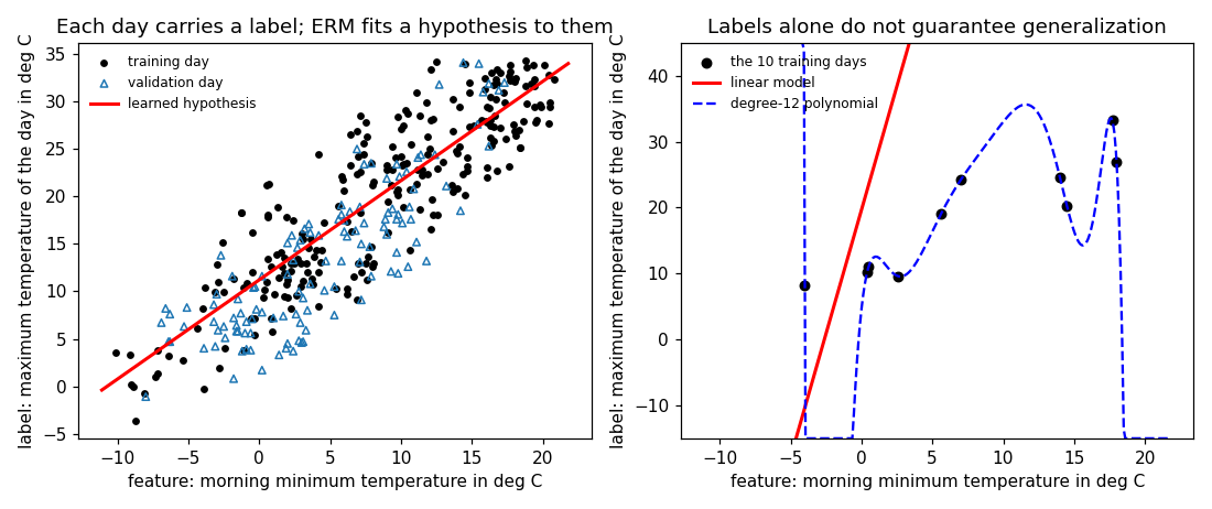
[B-plot]     Preview: the labeled days with the learned hypothesis, and
             the overfitting polynomial beside it.

Outputs
-------
supervisedlearning_weather.csv : date, tmin, tmax for the 366 days
supervisedlearning_train.csv   : x, y of the training days
supervisedlearning_val.csv     : x, y of the validation days
supervisedlearning_fit.csv     : x, linear, poly -- the two hypotheses
supervisedlearning.png         : preview (checking only)
"""

import json
import urllib.request
from pathlib import Path

import numpy as np
import matplotlib

matplotlib.use("Agg")
import matplotlib.pyplot as plt

OUT_DIR = Path(__file__).parent

report = []


def check(name, ok):
    report.append((name, bool(ok)))
    print(f"  [{'ok' if ok else 'FAIL'}] {name}")
Download the 366 daily temperature pairs at Krems for 2024; feature = morning minimum, label = maximum of the day; split into a training set (January to August) and a validation set (September to December).
URL = ("https://dataset.api.hub.geosphere.at/v1/station/historical/"
       "klima-v2-1d?parameters=tlmin,tlmax&station_ids=3805"
       "&start=2024-01-01&end=2024-12-31")
with urllib.request.urlopen(URL, timeout=120) as resp:
    payload = json.load(resp)
params = payload["features"][0]["properties"]["parameters"]
stamps = [t[:10] for t in payload["timestamps"]]
tmin = np.array(params["tlmin"]["data"], dtype=float)
tmax = np.array(params["tlmax"]["data"], dtype=float)
with open(OUT_DIR / "supervisedlearning_weather.csv", "w") as f:
    f.write("date,tmin,tmax\n")
    for day, lo, hi in zip(stamps, tmin, tmax):
        f.write(f"{day},{lo},{hi}\n")
check("[B-data] 366 labeled days downloaded for 2024", len(tmin) == 366)
check("[B-data] the record matches the archive (Feb 1: -3.8 to 10.4 deg)",
      stamps[31] == "2024-02-01" and np.isclose(tmin[31], -3.8)
      and np.isclose(tmax[31], 10.4))

x, y = tmin, tmax                              # feature, label
train = np.arange(len(x)) < 244                # January to August
val = ~train                                   # September to December
check("[B-data] every data point carries a label", len(x) == len(y))
check("[B-data] 244 training days and 122 validation days",
      train.sum() == 244 and val.sum() == 122)


def lstsq_fit(xs, ys, degree):
    """ERM over the polynomials of the given degree, squared error loss."""
    A = np.vander(xs, degree + 1)
    return np.linalg.lstsq(A, ys, rcond=None)[0]


def mse(w, xs, ys):
    return float(np.mean((np.vander(xs, len(w)) @ w - ys) ** 2))
  [ok] [B-data] 366 labeled days downloaded for 2024
  [ok] [B-data] the record matches the archive (Feb 1: -3.8 to 10.4 deg)
  [ok] [B-data] every data point carries a label
  [ok] [B-data] 244 training days and 122 validation days
  linear model: training error 17.80, validation error 24.31; label variance 80.71, sample-mean baseline 108.06
ERM over the linear model on the training set; check the training error is far below the sample variance of the labels, that the validation error is close to the training error, and that both beat predicting the sample mean of the training labels.
w_lin = lstsq_fit(x[train], y[train], 1)
err_train = mse(w_lin, x[train], y[train])
err_val = mse(w_lin, x[val], y[val])
var_labels = float(np.var(y[train]))
err_mean = float(np.mean((y[train].mean() - y[val]) ** 2))
print(f"  linear model: training error {err_train:.2f}, validation error "
      f"{err_val:.2f}; label variance {var_labels:.2f}, sample-mean "
      f"baseline {err_mean:.2f}")
check("[B-erm] the training error is far below the sample variance of the "
      "labels", err_train < 0.35 * var_labels)
check("[B-erm] the validation error is close to the training error",
      err_val < 1.5 * err_train)
check("[B-erm] both beat predicting the sample mean of the training labels",
      err_val < 0.5 * err_mean)
  [ok] [B-erm] the training error is far below the sample variance of the labels
  [ok] [B-erm] the validation error is close to the training error
  [ok] [B-erm] both beat predicting the sample mean of the training labels
  degree-12 polynomial on 10 days: training error 0.0000, validation error 26790827; linear model on the same 10 days: 11.61 and 23.28
The same labels, a training set of ten days and a degree-12 polynomial: smaller training error, far larger validation error.
small = np.zeros(len(x), dtype=bool)
small[np.linspace(0, 243, 10).astype(int)] = True
xs = (x[small] - x[train].mean()) / x[train].std()     # scaled, for conditioning
xv = (x[val] - x[train].mean()) / x[train].std()
w_poly = lstsq_fit(xs, y[small], 12)
poly_train = mse(w_poly, xs, y[small])
poly_val = mse(w_poly, xv, y[val])
w_lin_small = lstsq_fit(xs, y[small], 1)
print(f"  degree-12 polynomial on 10 days: training error {poly_train:.4f}, "
      f"validation error {poly_val:.0f}; linear model on the same 10 days: "
      f"{mse(w_lin_small, xs, y[small]):.2f} and "
      f"{mse(w_lin_small, xv, y[val]):.2f}")
check("[B-overfit] the polynomial has a smaller training error than the "
      "linear model", poly_train < mse(w_lin_small, xs, y[small]))
check("[B-overfit] and a far larger validation error",
      poly_val > 10 * mse(w_lin_small, xv, y[val]))
  [ok] [B-overfit] the polynomial has a smaller training error than the linear model
  [ok] [B-overfit] and a far larger validation error
  classification: frost on 19% of the days; threshold 7.2 deg, validation accuracy 0.81 against the majority class 0.71
The label space decides the task: the binary label "frost in the morning" turns the same records into a classification problem; a threshold rule fitted by ERM with the zero-one loss beats predicting the majority class.
frost = (tmin < 0.0).astype(int)               # label constructed from tmin
feat = tmax                                    # feature: maximum of the day
thresholds = np.linspace(feat.min(), feat.max(), 400)
errs = [np.mean((feat[train] < t).astype(int) != frost[train])
        for t in thresholds]
t_hat = float(thresholds[int(np.argmin(errs))])
acc_val = float(np.mean((feat[val] < t_hat).astype(int) == frost[val]))
majority = float(max(frost[train].mean(), 1 - frost[train].mean()))
acc_major = float(np.mean(frost[val] == int(frost[train].mean() > 0.5)))
print(f"  classification: frost on {100 * frost.mean():.0f}% of the days; "
      f"threshold {t_hat:.1f} deg, validation accuracy {acc_val:.2f} against "
      f"the majority class {acc_major:.2f}")
check("[B-classify] the binary label splits the days into two nonempty "
      "classes", 0 < frost.sum() < len(frost))
check("[B-classify] the threshold rule beats the majority class",
      acc_val > acc_major)
check("[B-classify] both problems use the same data points, only the label "
      "space differs", len(feat) == len(y) and majority <= 1.0)

# ---- CSVs for the entry's figure
np.savetxt(OUT_DIR / "supervisedlearning_train.csv",
           np.stack([x[train], y[train]], 1), delimiter=",",
           header="x,y", comments="", fmt="%.1f")
np.savetxt(OUT_DIR / "supervisedlearning_val.csv",
           np.stack([x[val], y[val]], 1), delimiter=",",
           header="x,y", comments="", fmt="%.1f")
grid = np.linspace(x.min() - 1, x.max() + 1, 300)
gs = (grid - x[train].mean()) / x[train].std()
with open(OUT_DIR / "supervisedlearning_fit.csv", "w") as f:
    f.write("x,linear,poly\n")
    lin = np.vander(grid, 2) @ w_lin
    pol = np.clip(np.vander(gs, 13) @ w_poly, -15.0, 45.0)
    for a, b, c in zip(grid, lin, pol):
        f.write(f"{a:.2f},{b:.2f},{c:.2f}\n")
  [ok] [B-classify] the binary label splits the days into two nonempty classes
  [ok] [B-classify] the threshold rule beats the majority class
  [ok] [B-classify] both problems use the same data points, only the label space differs

12/12 checks pass
Preview: the labeled days with the learned hypothesis, and the overfitting polynomial beside it.
fig, (ax1, ax2) = plt.subplots(1, 2, figsize=(10, 4.2))
ax1.scatter(x[train], y[train], s=12, color="black", label="training day")
ax1.scatter(x[val], y[val], s=18, marker="^", facecolors="none",
            edgecolors="tab:blue", label="validation day")
ax1.plot(grid, np.vander(grid, 2) @ w_lin, "r-", lw=2,
         label="learned hypothesis")
ax1.set_xlabel("feature: morning minimum temperature in deg C")
ax1.set_ylabel("label: maximum temperature of the day in deg C")
ax1.set_title("Each day carries a label; ERM fits a hypothesis to them")
ax1.legend(frameon=False, fontsize=8)
ax2.scatter(x[small], y[small], s=30, color="black", label="the 10 training days")
ax2.plot(grid, np.vander(grid, 2) @ w_lin_small, "r-", lw=2, label="linear model")
ax2.plot(grid, np.clip(np.vander(gs, 13) @ w_poly, -15, 45), "b--", lw=1.5,
         label="degree-12 polynomial")
ax2.set_ylim(-15, 45)
ax2.set_xlabel("feature: morning minimum temperature in deg C")
ax2.set_ylabel("label: maximum temperature of the day in deg C")
ax2.set_title("Labels alone do not guarantee generalization")
ax2.legend(frameon=False, fontsize=8)
fig.tight_layout()
fig.savefig(OUT_DIR / "supervisedlearning.png", dpi=110)

n_ok = sum(ok for _, ok in report)
print(f"\n{n_ok}/{len(report)} checks pass")
if n_ok != len(report):
    raise SystemExit(1)
B-plot writes when the script runs