B-minibatch writes when the script runsDictionary of Applied Machine Learning · stochastic gradient descent (SGD)
Numerical companion to the entry stochastic gradient descent (SGD): it recomputes what the entry states and prints one line per check
One block per claim/figure of the entry (marked [B-...], linked from the entry's paragraphs by content): each block verifies numerically what the corresponding statement asserts or generates the data behind a figure. Fixed seeds; numpy/matplotlib plus stdlib urllib for the one-time download of the weather observations behind Fig. 1 (cached in the committed CSVs — re-runs read those and need no network).
Run it without installing anything:uv run https://dictionaryofml.org/terms/stochGD.py
uv downloads this script and the pinned NumPy and Matplotlib it needs, then runs it; the script fetches any input file it uses. To keep the output files, download stochGD.py into a folder and run uv run stochGD.py there. With NumPy and Matplotlib already installed, python3 stochGD.py, from any directory — it writes its output files into the current directory. Fixed seeds, so the printed numbers reproduce exactly. Download stochGD.py · Notebook · Open in Colab
One cell per block of the script: the code, and what that code printed when it last ran here
"""
stochGD.py — numerical companion to the glossary entry
'stochastic gradient descent (SGD)'.

One block per claim/figure of the entry (marked [B-...], linked from the
entry's paragraphs by content): each block verifies numerically what the
corresponding statement asserts or generates the data behind a figure.
Fixed seeds; numpy/matplotlib plus stdlib urllib for the one-time
download of the weather observations behind Fig. 1 (cached in the
committed CSVs — re-runs read those and need no network).

Blocks
------
[B-weather]   Real training set behind Fig. 1 of the entry: daily
              minimum temperature (feature x) and daily maximum
              temperature (label y) observed on 2026-07-01 at 6 Austrian
              weather stations (downloaded from the GeoSphere Austria
              open data API, dataset klima-v2-1d) and 6 Finnish stations
              (downloaded from the FMI open data WFS, daily
              observations). A linear hypothesis map h(x) = w1 x + w0 is
              learned by ERM on the m = 12 data points; a fixed random
              subset of 4 data points is the batch that one SGD update
              uses in place of the full training set.
[B-approx]    SGD replaces the full gradient — a sum of per-data-point
              gradients over the entire trainset — with the sum over a
              randomly chosen batch: the batch gradient is an unbiased
              approximation (its average over many random batches
              matches the full gradient), and one SGD step touches only
              |B| of the m data points.
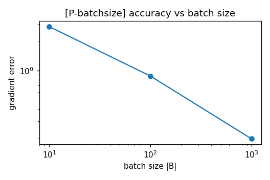
[B-batchsize] The batch size trades gradient accuracy against cost: the
              approximation error of the batch gradient shrinks like
              1/sqrt(|B|) as the batch grows (variance scaling), while
              the per-step cost grows linearly in |B|.
[B-minibatch] Mini-batch SGD (|B| > 1) converges to the ERM solution on
              a least-squares problem while evaluating only a small
              fraction of the per-data-point gradients that full GD
              uses for the same number of passes.

Outputs
-------
stochGD_geosphere.csv  : tmin, tmax — the 6 Austrian data points.
stochGD_fmi.csv        : tmin, tmax — the 6 Finnish data points.
stochGD_batch.csv      : tmin, tmax — the 4 data points of the batch.
stochGD_hypothesis.csv : tmin, tmax — endpoints of the learned h(x).
stochGD_errorsegs.csv  : x, y — prediction-error segments (one segment
                         per data point, nan-separated for pgfplots
                         'unbounded coords=jump').
stochGD.png            : preview figure (checking only).

Data generated by pythondemos/stochGD.py.
"""

import numpy as np
import matplotlib

matplotlib.use("Agg")
import matplotlib.pyplot as plt
from pathlib import Path

OUT_DIR = Path(__file__).parent

rng = np.random.default_rng(42)
report = []


def check(name, ok):
    report.append((name, bool(ok)))
    print(f"  [{'ok' if ok else 'FAIL'}] {name}")


# least-squares ERM objective on m data points
m, d = 2000, 5
X = rng.normal(size=(m, d))
w_true = rng.normal(size=d)
y = X @ w_true + 0.3 * rng.normal(size=m)
full_grad = lambda w: (2 / m) * X.T @ (X @ w - y)
def batch_grad(w, B):
    idx = rng.choice(m, B, replace=False)
    return (2 / B) * X[idx].T @ (X[idx] @ w - y[idx]), B
Real training set behind Fig. 1 of the entry: daily minimum temperature (feature x) and daily maximum temperature (label y) observed on 2026-07-01 at 6 Austrian weather stations (downloaded from the GeoSphere Austria open data API, dataset klima-v2-1d) and 6 Finnish stations (downloaded from the FMI open data WFS, daily observations). A linear hypothesis map h(x) = w1 x + w0 is learned by ERM on the m = 12 data points; a fixed random subset of 4 data points is the batch that one SGD update uses in place of the full training set.
print("[B-weather] real tmin/tmax data points behind Fig. 1 of the entry")
DATE = "2026-07-01"
GEO_STATIONS = {105: "Wien Hohe Warte", 30: "Graz Universitaet",
39: "Innsbruck Universitaet", 48: "Klagenfurt Flughafen",
131: "Salzburg Flughafen", 5000: "Linz Hoersching"}
FMI_PLACES = ["Helsinki", "Tampere", "Turku", "Oulu", "Rovaniemi",
"Kuopio"]
def download_geosphere():
"""One (tmin, tmax) pair per Austrian station for DATE."""
import json
from urllib.request import urlopen
ids = ",".join(str(s) for s in GEO_STATIONS)
url = ("https://dataset.api.hub.geosphere.at/v1/station/historical/"
f"klima-v2-1d?parameters=tlmin,tlmax&station_ids={ids}"
f"&start={DATE}&end={DATE}")
feats = json.load(urlopen(url, timeout=60))["features"]
return sorted(
(f["properties"]["parameters"]["tlmin"]["data"][0],
f["properties"]["parameters"]["tlmax"]["data"][0])
for f in feats)
def download_fmi():
"""One (tmin, tmax) pair per Finnish place for DATE."""
import re
from urllib.request import urlopen
pairs = []
for place in FMI_PLACES:
url = ("https://opendata.fmi.fi/wfs?service=WFS&version=2.0.0"
"&request=getFeature&storedquery_id="
"fmi::observations::weather::daily::simple"
f"&place={place}&starttime={DATE}T00:00:00Z"
f"&endtime={DATE}T23:59:59Z¶meters=tmin,tmax")
xml = urlopen(url, timeout=60).read().decode()
vals = dict(re.findall(
r"<BsWfs:ParameterName>(\w+)</BsWfs:ParameterName>\s*"
r"<BsWfs:ParameterValue>([-\d.]+)</BsWfs:ParameterValue>",
xml))
pairs.append((float(vals["tmin"]), float(vals["tmax"])))
return sorted(pairs)
def write_csv(name, header, rows):
with open(OUT_DIR / name, "w") as f:
f.write(header + "\n")
for row in rows:
f.write(",".join(row) + "\n")
def read_csv(name):
lines = (OUT_DIR / name).read_text().strip().splitlines()[1:]
return [tuple(float(v) for v in ln.split(",")) for ln in lines]
try: # one-time download ...
geo, fmi = download_geosphere(), download_fmi()
write_csv("stochGD_geosphere.csv", "tmin,tmax",
[(f"{a:.1f}", f"{b:.1f}") for a, b in geo])
write_csv("stochGD_fmi.csv", "tmin,tmax",
[(f"{a:.1f}", f"{b:.1f}") for a, b in fmi])
print(f" downloaded {len(geo)}+{len(fmi)} stations for {DATE}")
except OSError as err: # ... offline: reuse committed CSVs
print(f" download failed ({err}); reading committed CSVs")
geo = read_csv("stochGD_geosphere.csv")
fmi = read_csv("stochGD_fmi.csv")
pts = geo + fmi # the training set, m = 12
x_all = np.array([p[0] for p in pts])
y_all = np.array([p[1] for p in pts])
# linear hypothesis h(x) = w1 x + w0 learned by ERM (average squared
# prediction error) on all m data points
fit_w1, fit_w0 = np.polyfit(x_all, y_all, 1)
yhat = fit_w1 * x_all + fit_w0
xg = (np.floor(x_all.min()) - 1.0, np.ceil(x_all.max()) + 1.0)
write_csv("stochGD_hypothesis.csv", "tmin,tmax",
[(f"{x:.1f}", f"{fit_w1 * x + fit_w0:.2f}") for x in xg])
# prediction-error segments, nan-separated for pgfplots
seg_rows = []
for xi, yi, hi in zip(x_all, y_all, yhat):
seg_rows += [(f"{xi:.1f}", f"{yi:.1f}"), (f"{xi:.1f}", f"{hi:.2f}"),
("nan", "nan")]
write_csv("stochGD_errorsegs.csv", "x,y", seg_rows)
# the batch: a fixed random subset of 4 of the m = 12 data points
batch_idx = np.sort(np.random.default_rng(1).choice(len(pts), 4,
replace=False))
write_csv("stochGD_batch.csv", "tmin,tmax",
[(f"{x_all[i]:.1f}", f"{y_all[i]:.1f}") for i in batch_idx])
check("6 Austrian + 6 Finnish data points (tmin, tmax) for " + DATE,
len(geo) == 6 and len(fmi) == 6)
check("the batch is a strict random subset of the training set",
0 < len(batch_idx) < len(pts))
check("the batch holds data points from both servers",
batch_idx.min() < len(geo) <= batch_idx.max())
check("ERM residuals of the linear hypothesis average to zero",
abs(np.mean(y_all - yhat)) < 1e-8)
[B-weather] real tmin/tmax data points behind Fig. 1 of the entry
    downloaded 6+6 stations for 2026-07-01
  [ok] 6 Austrian + 6 Finnish data points (tmin, tmax) for 2026-07-01
  [ok] the batch is a strict random subset of the training set
  [ok] the batch holds data points from both servers
  [ok] ERM residuals of the linear hypothesis average to zero
SGD replaces the full gradient — a sum of per-data-point gradients over the entire trainset — with the sum over a randomly chosen batch: the batch gradient is an unbiased approximation (its average over many random batches matches the full gradient), and one SGD step touches only |B| of the m data points.
print("[B-approx] the batch gradient approximates the full-sum gradient")
w0 = np.zeros(d)
g_full = full_grad(w0)
g_avg = np.mean([batch_grad(w0, 20)[0] for _ in range(4000)], axis=0)
check("averaging batch gradients over many draws recovers the full "
      "gradient (unbiasedness)",
      np.linalg.norm(g_avg - g_full) < 0.05 * np.linalg.norm(g_full))
check("one SGD step touches |B| = 20 of the m = 2000 data points",
      batch_grad(w0, 20)[1] == 20 < m)
[B-approx] the batch gradient approximates the full-sum gradient
  [ok] averaging batch gradients over many draws recovers the full gradient (unbiasedness)
  [ok] one SGD step touches |B| = 20 of the m = 2000 data points
The batch size trades gradient accuracy against cost: the approximation error of the batch gradient shrinks like 1/sqrt(|B|) as the batch grows (variance scaling), while the per-step cost grows linearly in |B|.
print("[B-batchsize] batch size trades accuracy against cost")
errs = []
for B in (10, 100, 1000):
    errs.append(np.mean([np.linalg.norm(batch_grad(w0, B)[0] - g_full)
                         for _ in range(300)]))
print(f"    mean gradient error at |B| = 10, 100, 1000: "
      f"{errs[0]:.3f}, {errs[1]:.3f}, {errs[2]:.3f}")
check("the gradient error shrinks as the batch grows",
      errs[0] > errs[1] > errs[2])
check("error scaling is consistent with 1/sqrt(|B|) "
      "(10x batch -> ~3.2x smaller error)",
      2.0 < errs[0] / errs[1] < 5.0 and 2.0 < errs[1] / errs[2] < 5.0)
[B-batchsize] batch size trades accuracy against cost
    mean gradient error at |B| = 10, 100, 1000: 2.813, 0.875, 0.199
  [ok] the gradient error shrinks as the batch grows
  [ok] error scaling is consistent with 1/sqrt(|B|) (10x batch -> ~3.2x smaller error)
Mini-batch SGD (|B| > 1) converges to the ERM solution on a least-squares problem while evaluating only a small fraction of the per-data-point gradients that full GD uses for the same number of passes.
print("[B-minibatch] mini-batch SGD reaches the ERM solution cheaply")
w_hat = np.linalg.solve(X.T @ X, X.T @ y)          # ERM solution
w = np.zeros(d)
grads_evaluated = 0
for t in range(1, 1201):
    g, B = batch_grad(w, 20)
    w -= (0.05 / np.sqrt(t)) * g
    grads_evaluated += B
gd_grads = 1200 * m                                 # full GD, same steps
check("mini-batch SGD converges near the ERM solution",
      np.linalg.norm(w - w_hat) < 0.1)
check("using 1% of the per-data-point gradient evaluations of full GD",
      grads_evaluated == 0.01 * gd_grads)

# ------------------------------------------------------------ preview
fig, (ax0, ax1) = plt.subplots(1, 2, figsize=(9.6, 3.4))
gx = np.array(xg)
ax0.plot(gx, fit_w1 * gx + fit_w0, "-", color="tab:blue",
         label="hypothesis h(x)")
for xi, yi, hi in zip(x_all, y_all, yhat):
    ax0.plot([xi, xi], [yi, hi], ":", color="gray", lw=1)
ax0.plot([p[0] for p in geo], [p[1] for p in geo], "o", color="black",
         label="stored at Geosphere.at")
ax0.plot([p[0] for p in fmi], [p[1] for p in fmi], "s", color="black",
         label="stored at FMI.fi")
ax0.plot(x_all[batch_idx], y_all[batch_idx], "o", mfc="none",
         mec="tab:red", ms=12, label="batch")
ax0.set_xlabel("daily minimum temperature (deg C)")
ax0.set_ylabel("daily maximum temperature (deg C)")
ax0.set_title(f"[B-weather] trainset, batch and errors ({DATE})")
ax0.legend(frameon=False, fontsize=8)
ax1.loglog([10, 100, 1000], errs, "o-")
ax1.set_xlabel("batch size |B|"); ax1.set_ylabel("gradient error")
ax1.set_title("[B-batchsize] accuracy vs batch size")
fig.tight_layout()
fig.savefig(OUT_DIR / "stochGD.png", dpi=110)
print(f"\n{sum(ok for _, ok in report)}/{len(report)} checks passed")
assert all(ok for _, ok in report)
[B-minibatch] mini-batch SGD reaches the ERM solution cheaply
  [ok] mini-batch SGD converges near the ERM solution
  [ok] using 1% of the per-data-point gradient evaluations of full GD

10/10 checks passed
B-minibatch writes when the script runs