B-plot writes when the script runsDictionary of Applied Machine Learning · spectral clustering
Updated on 2026-11-19
Numerical companion to the entry spectral clustering: it recomputes what the entry states and prints one line per check
Numerical companion to the glossary entry 'specclustering'. The 366 days of 2024 at Krems are data points with the feature vector (morning minimum temperature, maximum daytime temperature). Each day is a node of a graph and is connected to its ten nearest days in Euclidean distance; the edges have unit weight. Spectral clustering reads the clusters off the eigenvectors of the Laplacian matrix of this graph.
Run it without installing anything:uv run https://dictionaryofml.org/terms/specclustering.py
uv downloads this script and the pinned NumPy and Matplotlib it needs, then runs it; the script fetches any input file it uses. To keep the output files, download specclustering.py into a folder and run uv run specclustering.py there. With NumPy and Matplotlib already installed, python3 specclustering.py, from any directory — it writes its output files into the current directory. Fixed seeds, so the printed numbers reproduce exactly. Download specclustering.py · Notebook · Open in Colab
Before running a downloaded copy, scan it: uvx bandit -q -t B102,B307,B602,B605 specclustering.py (B102,B307,B602,B605 are the exec, eval and shell checks of bandit) reports nothing: the script runs no shell command and evaluates no generated code.
One cell per block of the script: the code, and what that code printed when it last ran here
"""Spectral clustering of the days of one year at Krems an der Donau:
the eigenvectors of the Laplacian matrix of their nearest-neighbor graph.

Purpose
-------
Numerical companion to the glossary entry 'specclustering'.  The 366
days of 2024 at Krems are data points with the feature vector (morning
minimum temperature, maximum daytime temperature).  Each day is a node
of a graph and is connected to its ten nearest days in Euclidean
distance; the edges have unit weight.  Spectral clustering reads the
clusters off the eigenvectors of the Laplacian matrix of this graph.

The demo checks the entry's claims: the Laplacian matrix is symmetric
and positive semi-definite, its quadratic form sums the squared
differences over the edges, its rows sum to zero, and the multiplicity
of its eigenvalue 0 is the number of connected components; the second
eigenvector (the Fiedler vector) of the connected graph has entries of
both signs, and k-means on the first k eigenvector entries delivers the
clusters; the ratio cut of every bipartition is at least the second
eigenvalue, the value of the relaxed problem that the Fiedler vector
solves; and on these data, whose clusters are convex, spectral
clustering and k-means on the raw feature vectors agree on most days.

Deterministic: k-means starts from fixed data points, the eigenvectors
come from numpy.linalg.eigh with their signs fixed.
Self-contained: numpy + matplotlib only; the GeoSphere download falls
back to the committed CSV.

Blocks
------
[B-data]      Download the daily minimum and maximum temperature of 2024
              at Krems (GeoSphere station 3805) or read the committed
              copy; 366 days, no missing value.
[B-graph]     The 10-nearest-neighbor graph of the days with unit edge
              weights, its Laplacian matrix L = D - A: symmetric, rows
              summing to zero, quadratic form equal to the sum of squared
              differences over the edges, hence positive semi-definite.
[B-spectrum]  Eigenvalues 0 = lambda_1 < lambda_2 <= ...: the graph is
              connected, so 0 is a simple eigenvalue with the constant
              eigenvector; the Fiedler vector has entries of both signs.
[B-cluster]   Spectral clustering with k = 2: k-means on the rows of the
              first two eigenvectors, which equals thresholding the
              Fiedler vector; the clusters are the cold and the warm
              days; agreement with k-means on the raw feature vectors.
[B-ratiocut]  The ratio cut of the spectral bipartition, of the k-means
              bipartition and of a random one, all at least lambda_2,
              the value of the relaxed problem.
[B-components] Deleting the edges between the two spectral clusters
              leaves two connected components: eigenvalue 0 then has
              multiplicity 2 and its eigenvectors are spanned by the two
              indicator vectors.
[B-three]     Spectral clustering with k = 3 from the first three
              eigenvectors: cluster sizes and connectivity in the graph.
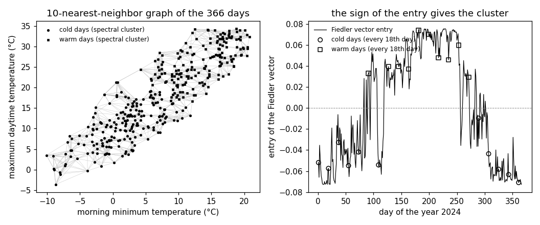
[B-plot]      The graph in the feature plane, every 18th day for the
              Fiedler-vector panel (21 of 366 days), and the preview.

Outputs
-------
specclustering_weather.csv : date, tmin, tmax (committed copy).
specclustering_nodes.csv   : every day with its features, day of the
                             year, spectral cluster, and Fiedler entry.
specclustering_edges.csv   : the edges of the graph as line segments,
                             separated by nan rows.
specclustering_fiedler.csv : Fiedler entry against day of the year.
specclustering_plot.csv    : the 21 drawn days with their cluster.
specclustering.png         : matplotlib preview (checking only).
"""

# /// script
# requires-python = ">=3.10"
# dependencies = ["matplotlib==3.10.7", "numpy==2.3.4"]
# ///

import json
import urllib.request
from pathlib import Path

import numpy as np
import matplotlib

matplotlib.use("Agg")
import matplotlib.pyplot as plt

OUT_DIR = Path(__file__).parent

report = []


def check(name, ok):
    report.append((name, bool(ok)))
    print(f"  [{'ok' if ok else 'FAIL'}] {name}")
Download the daily minimum and maximum temperature of 2024 at Krems (GeoSphere station 3805) or read the committed copy; 366 days, no missing value.
print("[B-data] daily minimum and maximum temperature at Krems, 2024")
URL = ("https://dataset.api.hub.geosphere.at/v1/station/historical/"
       "klima-v2-1d?parameters=tlmin,tlmax&station_ids=3805"
       "&start=2024-01-01&end=2024-12-31")
CSV = OUT_DIR / "specclustering_weather.csv"
try:
    with urllib.request.urlopen(URL, timeout=120) as resp:
        payload = json.load(resp)
    params = payload["features"][0]["properties"]["parameters"]
    records = [(stamp[:10], lo, hi)
               for stamp, lo, hi in zip(payload["timestamps"],
                                        params["tlmin"]["data"],
                                        params["tlmax"]["data"])]
    with open(CSV, "w") as fh:
        fh.write("date,tmin,tmax\n")
        for day, lo, hi in records:
            fh.write(f"{day},{lo},{hi}\n")
    print(f"    downloaded {len(records)} days")
except OSError as err:
    print(f"    download failed ({err}); reading the committed CSV")
    rows = CSV.read_text().strip().splitlines()[1:]
    records = [(d, float(a), float(b))
               for d, a, b in (r.split(",") for r in rows)]

check("[B-data] 366 days for 2024", len(records) == 366)
check("[B-data] no day is missing a temperature",
      all(lo is not None and hi is not None for _, lo, hi in records))
X = np.array([[lo, hi] for _, lo, hi in records], dtype=float)
dates = [d for d, _, _ in records]
months = np.array([int(d[5:7]) for d in dates])
n = len(X)
[B-data] daily minimum and maximum temperature at Krems, 2024
    downloaded 366 days
  [ok] [B-data] 366 days for 2024
  [ok] [B-data] no day is missing a temperature
The 10-nearest-neighbor graph of the days with unit edge weights, its Laplacian matrix L = D - A: symmetric, rows summing to zero, quadratic form equal to the sum of squared differences over the edges, hence positive semi-definite.
print("[B-graph] 10-nearest-neighbor graph of the days, Laplacian L = D - A")
NEIGHBORS = 10
dist = np.sqrt(((X[:, None, :] - X[None, :, :]) ** 2).sum(axis=2))
np.fill_diagonal(dist, np.inf)
nearest = np.argsort(dist, axis=1)[:, :NEIGHBORS]
A = np.zeros((n, n))
A[np.repeat(np.arange(n), NEIGHBORS), nearest.ravel()] = 1.0
A = np.maximum(A, A.T)                       # edge if either is a neighbor
edges = np.array([(i, j) for i in range(n) for j in range(i + 1, n)
                  if A[i, j] > 0])
deg = A.sum(axis=1)
L = np.diag(deg) - A
n_edges = len(edges)
check(f"[B-graph] {n} nodes, {n_edges} edges of unit weight, node degrees "
      f"between {int(deg.min())} and {int(deg.max())}",
      n_edges == int(A.sum() // 2) and deg.min() >= NEIGHBORS)
check("[B-graph] L is symmetric", np.array_equal(L, L.T))
check("[B-graph] every row of L sums to zero: L 1 = 0",
      np.allclose(L @ np.ones(n), 0.0))
rng = np.random.default_rng(3805)
u = rng.standard_normal(n)
quad = u @ L @ u
over_edges = ((u[edges[:, 0]] - u[edges[:, 1]]) ** 2).sum()
check("[B-graph] u^T L u equals the sum over the edges of (u_i - u_i')^2 "
      "for a random u", np.isclose(quad, over_edges))
lam, V = np.linalg.eigh(L)
check("[B-graph] L is positive semi-definite: all eigenvalues are "
      "nonnegative", lam.min() > -1e-9)


def components(adj, mask=None):
    """Number of connected components of the graph restricted to mask."""
    keep = np.ones(len(adj), bool) if mask is None else mask
    seen = ~keep
    count = 0
    for start in np.flatnonzero(keep):
        if seen[start]:
            continue
        count += 1
        stack = [start]
        seen[start] = True
        while stack:
            v = stack.pop()
            for w in np.flatnonzero(adj[v] > 0):
                if not seen[w]:
                    seen[w] = True
                    stack.append(w)
    return count
[B-graph] 10-nearest-neighbor graph of the days, Laplacian L = D - A
  [ok] [B-graph] 366 nodes, 2209 edges of unit weight, node degrees between 10 and 18
  [ok] [B-graph] L is symmetric
  [ok] [B-graph] every row of L sums to zero: L 1 = 0
  [ok] [B-graph] u^T L u equals the sum over the edges of (u_i - u_i')^2 for a random u
  [ok] [B-graph] L is positive semi-definite: all eigenvalues are nonnegative
Eigenvalues 0 = lambda_1 < lambda_2 <= ...: the graph is connected, so 0 is a simple eigenvalue with the constant eigenvector; the Fiedler vector has entries of both signs.
print("[B-spectrum] eigenvalues of L and the Fiedler vector")
check(f"[B-spectrum] lambda_1 = {lam[0]:.1e} is zero and lambda_2 = "
      f"{lam[1]:.3f} is positive: the graph is connected",
      abs(lam[0]) < 1e-9 and lam[1] > 1e-6 and components(A) == 1)
check("[B-spectrum] the eigenvector of lambda_1 is constant",
      np.allclose(V[:, 0], V[0, 0]))
fiedler = V[:, 1].copy()
cold_ref = int(np.argmin(X[:, 1]))             # the day with the lowest tmax
if fiedler[cold_ref] > 0:                      # the sign of an eigenvector
    fiedler = -fiedler                         # is arbitrary; cold days < 0
V[:, 1] = fiedler
check(f"[B-spectrum] the Fiedler vector is orthogonal to 1 and has "
      f"{int((fiedler < 0).sum())} negative and {int((fiedler > 0).sum())} "
      f"positive entries",
      abs(fiedler.sum()) < 1e-9 and (fiedler < 0).any() and (fiedler > 0).any())
check(f"[B-spectrum] lambda_2 = {lam[1]:.3f} lies well below lambda_3 = "
      f"{lam[2]:.3f}", lam[1] < 0.75 * lam[2])


def lloyd(Y, centroids):
    """Lloyd's algorithm from given centroids; returns labels, centroids,
    and the number of iterations until the assignment stops changing."""
    labels = None
    for it in range(1, 1000):
        d2 = ((Y[:, None, :] - centroids[None, :, :]) ** 2).sum(axis=2)
        new = np.argmin(d2, axis=1)
        if labels is not None and np.array_equal(new, labels):
            return labels, centroids, it
        labels = new
        centroids = np.vstack([Y[labels == c].mean(axis=0)
                               for c in range(len(centroids))])
    return labels, centroids, it


def farthest_first(Y, k, start):
    """Deterministic start: a given point, then always the farthest one."""
    chosen = [start]
    for _ in range(k - 1):
        d2 = ((Y[:, None, :] - Y[chosen]) ** 2).sum(axis=2).min(axis=1)
        chosen.append(int(d2.argmax()))
    return Y[chosen]


def ratio_cut(labels, adj):
    """Sum over the clusters of cut(C, V \\ C) / |C|."""
    total = 0.0
    for c in np.unique(labels):
        inside = labels == c
        total += adj[inside][:, ~inside].sum() / inside.sum()
    return total


def cut_size(labels, adj):
    """Total weight of the edges with endpoints in different clusters."""
    return sum(adj[labels == c][:, labels != c].sum()
               for c in np.unique(labels)) / 2
[B-spectrum] eigenvalues of L and the Fiedler vector
  [ok] [B-spectrum] lambda_1 = 1.0e-15 is zero and lambda_2 = 0.044 is positive: the graph is connected
  [ok] [B-spectrum] the eigenvector of lambda_1 is constant
  [ok] [B-spectrum] the Fiedler vector is orthogonal to 1 and has 190 negative and 176 positive entries
  [ok] [B-spectrum] lambda_2 = 0.044 lies well below lambda_3 = 0.179
Spectral clustering with k = 2: k-means on the rows of the first two eigenvectors, which equals thresholding the Fiedler vector; the clusters are the cold and the warm days; agreement with k-means on the raw feature vectors.
print("[B-cluster] spectral clustering with k = 2")
K = 2
Y2 = V[:, :K]                                  # new feature vector per node
start = farthest_first(Y2, K, int(np.argmin(fiedler)))
lab_sp, cent_sp, it_sp = lloyd(Y2, start)
if lab_sp[cold_ref] != 0:
    lab_sp = 1 - lab_sp
sign_part = (fiedler > 0).astype(int)
check(f"[B-cluster] k-means on the rows of (v1, v2) stops after {it_sp} "
      f"iterations and agrees with the sign of the Fiedler vector on "
      f"{100 * np.mean(lab_sp == sign_part):.1f}% of the days",
      np.mean(lab_sp == sign_part) > 0.97)
n_cold, n_warm = int((lab_sp == 0).sum()), int((lab_sp == 1).sum())
cold_months = sorted(set(months[lab_sp == 0]))
warm_months = sorted(set(months[lab_sp == 1]))
all_cold = [mth for mth in range(1, 13) if np.all(lab_sp[months == mth] == 0)]
all_warm = [mth for mth in range(1, 13) if np.all(lab_sp[months == mth] == 1)]
mean_cold, mean_warm = X[lab_sp == 0].mean(axis=0), X[lab_sp == 1].mean(axis=0)
check(f"[B-cluster] {n_cold} cold days with mean features "
      f"({mean_cold[0]:.1f}, {mean_cold[1]:.1f}) and {n_warm} warm days with "
      f"({mean_warm[0]:.1f}, {mean_warm[1]:.1f}); months entirely cold: "
      f"{all_cold}, entirely warm: {all_warm}",
      mean_cold[1] < mean_warm[1] and 1 in all_cold and 7 in all_warm)
check("[B-cluster] each spectral cluster is connected in the graph",
      components(A, lab_sp == 0) == 1 and components(A, lab_sp == 1) == 1)
# k-means on the raw feature vectors, started from the colder and the
# warmer half of the days as in the clusteringerror demo
order = np.argsort(X[:, 1])
start_raw = np.vstack([X[order[:n // 2]].mean(axis=0),
                       X[order[n // 2:]].mean(axis=0)])
lab_km, cent_km, it_km = lloyd(X, start_raw)
if cent_km[0, 1] > cent_km[1, 1]:
    lab_km = 1 - lab_km
agree = np.mean(lab_km == lab_sp)
check(f"[B-cluster] k-means on the raw feature vectors ({it_km} iterations) "
      f"assigns {100 * agree:.1f}% of the days like spectral clustering; "
      f"{int((lab_km != lab_sp).sum())} days differ", agree > 0.9)
differ = np.flatnonzero(lab_km != lab_sp)
print(f"    days assigned differently: {[dates[i] for i in differ]}")
[B-cluster] spectral clustering with k = 2
  [ok] [B-cluster] k-means on the rows of (v1, v2) stops after 3 iterations and agrees with the sign of the Fiedler vector on 99.5% of the days
  [ok] [B-cluster] 192 cold days with mean features (1.5, 10.5) and 174 warm days with (13.5, 26.1); months entirely cold: [1, 2, 11, 12], entirely warm: [5, 6, 7, 8]
  [ok] [B-cluster] each spectral cluster is connected in the graph
  [ok] [B-cluster] k-means on the raw feature vectors (3 iterations) assigns 99.5% of the days like spectral clustering; 2 days differ
    days assigned differently: ['2024-10-08', '2024-10-27']
The ratio cut of the spectral bipartition, of the k-means bipartition and of a random one, all at least lambda_2, the value of the relaxed problem.
print("[B-ratiocut] ratio cut of bipartitions against lambda_2")
rng = np.random.default_rng(2024)
lab_rand = rng.integers(0, 2, size=n)
cuts = {"spectral": lab_sp, "k-means on raw features": lab_km,
        "random": lab_rand}
rc = {name: ratio_cut(lab, A) for name, lab in cuts.items()}
cs = {name: int(cut_size(lab, A)) for name, lab in cuts.items()}
for name in cuts:
    check(f"[B-ratiocut] {name}: {cs[name]} of the {n_edges} edges are "
          f"cut, ratio cut {rc[name]:.3f} >= lambda_2 = {lam[1]:.3f}",
          rc[name] >= lam[1] - 1e-12)
check("[B-ratiocut] the spectral bipartition has the smallest ratio cut "
      "of the three", rc["spectral"] <= min(rc.values()) + 1e-12)
# the two-valued vector of the relaxation identity
a, b = (lab_sp == 0).sum(), (lab_sp == 1).sum()
f = np.where(lab_sp == 0, np.sqrt(b / a), -np.sqrt(a / b))
check("[B-ratiocut] for the two-valued vector f of the spectral partition, "
      "f^T L f = n RatioCut, f is orthogonal to 1, and ||f||^2 = n",
      np.isclose(f @ L @ f, n * rc["spectral"]) and abs(f.sum()) < 1e-9
      and np.isclose(f @ f, n))
check(f"[B-ratiocut] the relaxed problem attains n lambda_2 = "
      f"{n * lam[1]:.1f} at the Fiedler vector scaled to norm sqrt(n), "
      f"below f^T L f = {f @ L @ f:.1f}",
      np.isclose(np.sqrt(n) * fiedler @ L @ (np.sqrt(n) * fiedler),
                 n * lam[1]) and n * lam[1] <= f @ L @ f)
[B-ratiocut] ratio cut of bipartitions against lambda_2
  [ok] [B-ratiocut] spectral: 25 of the 2209 edges are cut, ratio cut 0.274 >= lambda_2 = 0.044
  [ok] [B-ratiocut] k-means on raw features: 35 of the 2209 edges are cut, ratio cut 0.383 >= lambda_2 = 0.044
  [ok] [B-ratiocut] random: 1130 of the 2209 edges are cut, ratio cut 12.457 >= lambda_2 = 0.044
  [ok] [B-ratiocut] the spectral bipartition has the smallest ratio cut of the three
  [ok] [B-ratiocut] for the two-valued vector f of the spectral partition, f^T L f = n RatioCut, f is orthogonal to 1, and ||f||^2 = n
  [ok] [B-ratiocut] the relaxed problem attains n lambda_2 = 16.0 at the Fiedler vector scaled to norm sqrt(n), below f^T L f = 100.2
Deleting the edges between the two spectral clusters leaves two connected components: eigenvalue 0 then has multiplicity 2 and its eigenvectors are spanned by the two indicator vectors.
print("[B-components] deleting the cut edges: multiplicity of eigenvalue 0")
A_cut = A.copy()
between = lab_sp[edges[:, 0]] != lab_sp[edges[:, 1]]
for i, j in edges[between]:
    A_cut[i, j] = A_cut[j, i] = 0.0
L_cut = np.diag(A_cut.sum(axis=1)) - A_cut
lam_cut, V_cut = np.linalg.eigh(L_cut)
n_zero = int((np.abs(lam_cut) < 1e-9).sum())
check(f"[B-components] {components(A_cut)} connected components, eigenvalue "
      f"0 with multiplicity {n_zero}, lambda_3 = {lam_cut[2]:.3f} > 0",
      components(A_cut) == 2 and n_zero == 2 and lam_cut[2] > 1e-6)
ind = np.stack([(lab_sp == 0).astype(float), (lab_sp == 1).astype(float)],
               axis=1)
check("[B-components] the indicator vectors of the two components are "
      "eigenvectors of eigenvalue 0 and span its eigenspace",
      np.allclose(L_cut @ ind, 0.0)
      and np.allclose(V_cut[:, :2] @ (V_cut[:, :2].T @ ind), ind))
[B-components] deleting the cut edges: multiplicity of eigenvalue 0
  [ok] [B-components] 2 connected components, eigenvalue 0 with multiplicity 2, lambda_3 = 0.171 > 0
  [ok] [B-components] the indicator vectors of the two components are eigenvectors of eigenvalue 0 and span its eigenspace
Spectral clustering with k = 3 from the first three eigenvectors: cluster sizes and connectivity in the graph.
print("[B-three] spectral clustering with k = 3")
Y3 = V[:, :3]
lab3, _, it3 = lloyd(Y3, farthest_first(Y3, 3, int(np.argmin(fiedler))))
sizes3 = np.bincount(lab3, minlength=3)
order3 = np.argsort([X[lab3 == c, 1].mean() for c in range(3)])
lab3 = np.argsort(order3)[lab3]                # 0 = coldest, 2 = warmest
sizes3 = np.bincount(lab3, minlength=3)
means3 = [X[lab3 == c].mean(axis=0) for c in range(3)]
conn3 = sum(components(A, lab3 == c) == 1 for c in range(3))
check(f"[B-three] k-means on the rows of (v1, v2, v3) after {it3} iterations: "
      f"cluster sizes {sizes3.tolist()} with mean maximum temperatures "
      f"{means3[0][1]:.1f}, {means3[1][1]:.1f}, {means3[2][1]:.1f}; "
      f"{conn3} of 3 clusters connected in the graph",
      sizes3.min() > 20 and conn3 >= 2)
[B-three] spectral clustering with k = 3
  [ok] [B-three] k-means on the rows of (v1, v2, v3) after 7 iterations: cluster sizes [107, 170, 89] with mean maximum temperatures 7.1, 18.5, 29.8; 3 of 3 clusters connected in the graph
The graph in the feature plane, every 18th day for the Fiedler-vector panel (21 of 366 days), and the preview.
print("[B-plot] graph in the feature plane, Fiedler vector, preview")
doy = np.arange(1, n + 1)
with open(OUT_DIR / "specclustering_nodes.csv", "w") as fh:
    fh.write("date,doy,tmin,tmax,cluster,v2\n")
    for i in range(n):
        fh.write(f"{dates[i]},{doy[i]},{X[i, 0]:.1f},{X[i, 1]:.1f},"
                 f"{lab_sp[i]},{fiedler[i]:.5f}\n")
with open(OUT_DIR / "specclustering_edges.csv", "w") as fh:
    fh.write("tmin,tmax\n")
    for i, j in edges:
        fh.write(f"{X[i, 0]:.1f},{X[i, 1]:.1f}\n{X[j, 0]:.1f},{X[j, 1]:.1f}\n"
                 "nan,nan\n")
with open(OUT_DIR / "specclustering_fiedler.csv", "w") as fh:
    fh.write("doy,v2\n")
    for i in range(n):
        fh.write(f"{doy[i]},{fiedler[i]:.5f}\n")
idx = np.arange(0, n, 18)
with open(OUT_DIR / "specclustering_plot.csv", "w") as fh:
    fh.write("doy,tmin,tmax,cluster,v2\n")
    for i in idx:
        fh.write(f"{doy[i]},{X[i, 0]:.1f},{X[i, 1]:.1f},{lab_sp[i]},"
                 f"{fiedler[i]:.5f}\n")
check(f"[B-plot] every 18th day: {len(idx)} of the {n} days are drawn in "
      f"the Fiedler-vector panel", len(idx) == 21)
check(f"[B-plot] the edge file holds {n_edges} segments",
      sum(1 for _ in open(OUT_DIR / "specclustering_edges.csv")) - 1
      == 3 * n_edges)

fig, (ax1, ax2) = plt.subplots(1, 2, figsize=(9.6, 4.0))
for i, j in edges:
    ax1.plot([X[i, 0], X[j, 0]], [X[i, 1], X[j, 1]], color="0.75",
             lw=0.3, zorder=1)
for c, mk, lab in ((0, "o", "cold days"), (1, "s", "warm days")):
    sel = lab_sp == c
    ax1.scatter(X[sel, 0], X[sel, 1], marker=mk, s=9, facecolors="black",
                edgecolors="black", lw=0.4, zorder=2,
                label=f"{lab} (spectral cluster)")
ax1.set_xlabel("morning minimum temperature (°C)")
ax1.set_ylabel("maximum daytime temperature (°C)")
ax1.set_title(f"{NEIGHBORS}-nearest-neighbor graph of the {n} days")
ax1.legend(frameon=False, fontsize=8, loc="upper left")
ax2.plot(doy, fiedler, color="black", lw=0.8, label="Fiedler vector entry")
ax2.axhline(0.0, color="0.5", lw=0.6, ls="--")
for c, mk, lab in ((0, "o", "cold days"), (1, "s", "warm days")):
    sel = idx[lab_sp[idx] == c]
    ax2.scatter(doy[sel], fiedler[sel], marker=mk, facecolors="none",
                edgecolors="black", s=30, zorder=3,
                label=f"{lab} (every 18th day)")
ax2.set_xlabel("day of the year 2024")
ax2.set_ylabel("entry of the Fiedler vector")
ax2.set_title("the sign of the entry gives the cluster")
ax2.legend(frameon=False, fontsize=8, loc="upper left")
fig.tight_layout()
fig.savefig(OUT_DIR / "specclustering.png", dpi=110)

n_ok = sum(ok for _, ok in report)
print(f"\n{n_ok}/{len(report)} checks pass")
if n_ok != len(report):
    raise SystemExit(1)
[B-plot] graph in the feature plane, Fiedler vector, preview
  [ok] [B-plot] every 18th day: 21 of the 366 days are drawn in the Fiedler-vector panel
  [ok] [B-plot] the edge file holds 2209 segments

26/26 checks pass
B-plot writes when the script runs