B-logodds writes when the script runsDictionary of Applied Machine Learning · sigmoid function
Numerical companion to the entry sigmoid function: it recomputes what the entry states and prints one line per check
Checks the entry's claims about the sigmoid function sigma(z) = 1 / (1 + exp(-z)): its range, limits and symmetry; the closed form of its derivative, its maximum 1/4 and its vanishing for large |z|; and the log-odds reading, where sigma of a linear function of the feature vector is exactly the posterior probability of the label when the feature vectors of the two classes are Gaussian with one shared covariance matrix. Self-contained (numpy/matplotlib only), fixed seed.
Run it without installing anything:uv run https://dictionaryofml.org/terms/sigmoid.py
uv downloads this script and the pinned NumPy and Matplotlib it needs, then runs it; the script fetches any input file it uses. To keep the output files, download sigmoid.py into a folder and run uv run sigmoid.py there. With NumPy and Matplotlib already installed, python3 sigmoid.py, from any directory — it writes its output files into the current directory. Fixed seeds, so the printed numbers reproduce exactly. Download sigmoid.py · Notebook · Open in Colab
One cell per block of the script: the code, and what that code printed when it last ran here
"""
sigmoid.py — numerical companion to the glossary entry 'sigmoid function'.

Purpose
-------
Checks the entry's claims about the sigmoid function sigma(z) =
1 / (1 + exp(-z)): its range, limits and symmetry; the closed form of its
derivative, its maximum 1/4 and its vanishing for large |z|; and the
log-odds reading, where sigma of a linear function of the feature vector
is exactly the posterior probability of the label when the feature
vectors of the two classes are Gaussian with one shared covariance
matrix.  Self-contained (numpy/matplotlib only), fixed seed.

Blocks
------
[B-shape]   sigma maps the real line into (0, 1), tends to 0 and 1 at the
            two ends, passes through 1/2 at z = 0, is strictly increasing,
            and satisfies sigma(-z) = 1 - sigma(z).
[B-deriv]   sigma'(z) = sigma(z)(1 - sigma(z)) matches the slope of sigma
            measured between nearby points; it is at most 1/4, at z = 0,
            and at |z| = 10 it is below 1e-4: a neuron with a score of
            that size passes almost no gradient back.
[B-logodds] Two classes with Gaussian feature vectors sharing one
            covariance matrix: the posterior probability of the label 1
            equals sigma(a) for the log-odds a, a is a linear function
            w^T x + b of the feature vector, and log(sigma / (1 - sigma))
            recovers a.

Outputs
-------
sigmoid_curve.csv     : z, sigma(z), sigma'(z) on a grid
sigmoid_posterior.csv : feature vectors on a line through the feature
                        space, their log-odds, the posterior probability
                        of label 1 and sigma of the linear function
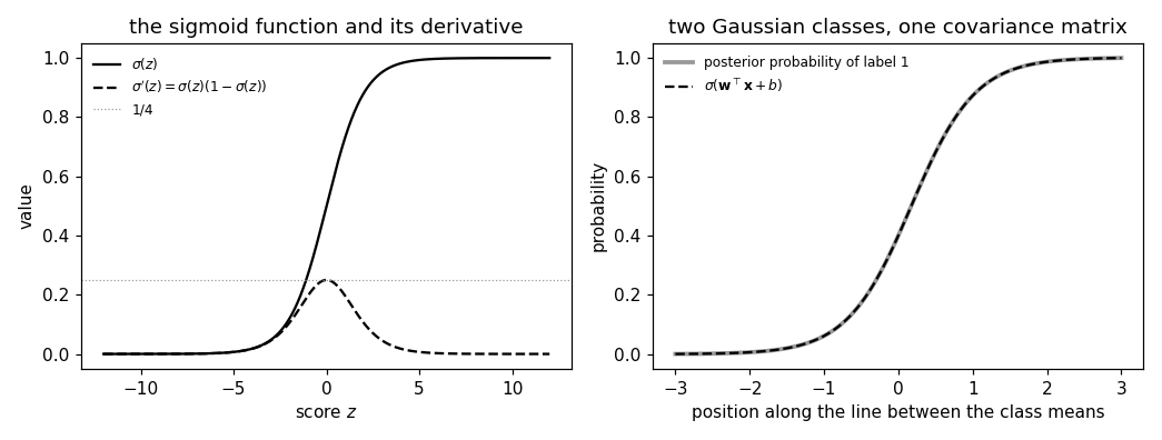
sigmoid.png           : matplotlib preview (checking only)
"""

import numpy as np
import matplotlib

matplotlib.use("Agg")
import matplotlib.pyplot as plt

from pathlib import Path

OUT_DIR = Path(__file__).parent

report = []


def check(name, ok):
    report.append((name, bool(ok)))
    print(f"  [{'ok' if ok else 'FAIL'}] {name}")


def sigma(z):
    return 1.0 / (1.0 + np.exp(-z))
sigma maps the real line into (0, 1), tends to 0 and 1 at the two ends, passes through 1/2 at z = 0, is strictly increasing, and satisfies sigma(-z) = 1 - sigma(z).
z = np.linspace(-12.0, 12.0, 2401)
s = sigma(z)
check(f"[B-shape]   sigma takes values in (0, 1): on [-12, 12] between {s.min():.2e} and "
      f"{s.max():.6f}", 0.0 < s.min() and s.max() < 1.0)
check(f"[B-shape]   sigma(-40) = {sigma(-40.0):.1e} and 1 - sigma(40) = {1 - sigma(40.0):.1e}: "
      "the two limits 0 and 1", sigma(-40.0) < 1e-15 and 1 - sigma(40.0) < 1e-15)
check("[B-shape]   sigma(0) = 1/2 and sigma is strictly increasing",
      sigma(0.0) == 0.5 and bool(np.all(np.diff(s) > 0)))
check(f"[B-shape]   sigma(-z) = 1 - sigma(z), to within {np.max(np.abs(sigma(-z) - (1 - s))):.1e}",
      np.max(np.abs(sigma(-z) - (1 - s))) < 1e-15)
  [ok] [B-shape]   sigma takes values in (0, 1): on [-12, 12] between 6.14e-06 and 0.999994
  [ok] [B-shape]   sigma(-40) = 4.2e-18 and 1 - sigma(40) = 0.0e+00: the two limits 0 and 1
  [ok] [B-shape]   sigma(0) = 1/2 and sigma is strictly increasing
  [ok] [B-shape]   sigma(-z) = 1 - sigma(z), to within 1.6e-16
sigma'(z) = sigma(z)(1 - sigma(z)) matches the slope of sigma measured between nearby points; it is at most 1/4, at z = 0, and at |z| = 10 it is below 1e-4: a neuron with a score of that size passes almost no gradient back.
ds = s * (1.0 - s)
slope = (sigma(z + 1e-5) - sigma(z - 1e-5)) / 2e-5
check(f"[B-deriv]   sigma'(z) = sigma(z)(1 - sigma(z)) matches the measured slope to within "
      f"{np.max(np.abs(ds - slope)):.1e}", np.max(np.abs(ds - slope)) < 1e-8)
check(f"[B-deriv]   the derivative is at most 1/4, reached at z = {z[np.argmax(ds)]:.2f}",
      abs(ds.max() - 0.25) < 1e-12 and z[np.argmax(ds)] == 0.0)
check(f"[B-deriv]   at |z| = 10 the derivative is {sigma(10.0) * (1 - sigma(10.0)):.1e}: almost "
      "no gradient passes back", sigma(10.0) * (1 - sigma(10.0)) < 1e-4)
with open(OUT_DIR / "sigmoid_curve.csv", "w") as fh:
    fh.write("z,sigma,derivative\n")
    for zi, si, di in zip(z[::20], s[::20], ds[::20]):
        fh.write(f"{zi:.2f},{si:.6f},{di:.6f}\n")
  [ok] [B-deriv]   sigma'(z) = sigma(z)(1 - sigma(z)) matches the measured slope to within 1.4e-11
  [ok] [B-deriv]   the derivative is at most 1/4, reached at z = 0.00
  [ok] [B-deriv]   at |z| = 10 the derivative is 4.5e-05: almost no gradient passes back
Two classes with Gaussian feature vectors sharing one covariance matrix: the posterior probability of the label 1 equals sigma(a) for the log-odds a, a is a linear function w^T x + b of the feature vector, and log(sigma / (1 - sigma)) recovers a.
# two classes in the plane, Gaussian feature vectors with one shared
# covariance matrix; the posterior probability of label 1 follows from the
# two densities and the class probabilities
rng = np.random.default_rng(0)
mu1, mu0 = np.array([1.5, 0.5]), np.array([-1.0, -0.5])
C = np.array([[1.0, 0.4], [0.4, 0.8]]); Cinv = np.linalg.inv(C)
p1 = 0.4                                            # probability of the label 1


def density(x, mu):
    d = x - mu
    return np.exp(-0.5 * np.einsum("ij,jk,ik->i", d, Cinv, d)) / (2 * np.pi * np.sqrt(np.linalg.det(C)))


w = Cinv @ (mu1 - mu0)
b = -0.5 * mu1 @ Cinv @ mu1 + 0.5 * mu0 @ Cinv @ mu0 + np.log(p1 / (1 - p1))
xs = rng.standard_normal((2000, 2)) * 1.5
logodds = np.log(density(xs, mu1) * p1) - np.log(density(xs, mu0) * (1 - p1))
posterior = density(xs, mu1) * p1 / (density(xs, mu1) * p1 + density(xs, mu0) * (1 - p1))
check(f"[B-logodds] the posterior probability of the label 1 equals sigma(a) for the log-odds a, "
      f"to within {np.max(np.abs(posterior - sigma(logodds))):.1e}",
      np.max(np.abs(posterior - sigma(logodds))) < 1e-12)
check(f"[B-logodds] with one shared covariance matrix the log-odds is linear, a = w^T x + b with "
      f"w = ({w[0]:.2f}, {w[1]:.2f}), b = {b:.2f}, to within "
      f"{np.max(np.abs(logodds - (xs @ w + b))):.1e}", np.max(np.abs(logodds - (xs @ w + b))) < 1e-10)
check("[B-logodds] log(sigma / (1 - sigma)) recovers the log-odds",
      np.max(np.abs(np.log(posterior / (1 - posterior)) - logodds)) < 1e-8)
t = np.linspace(-3.0, 3.0, 121)
line = np.outer(t, (mu1 - mu0) / np.linalg.norm(mu1 - mu0)) + (mu1 + mu0) / 2
post_line = density(line, mu1) * p1 / (density(line, mu1) * p1 + density(line, mu0) * (1 - p1))
with open(OUT_DIR / "sigmoid_posterior.csv", "w") as fh:
    fh.write("t,x1,x2,logodds,posterior,sigma_linear\n")
    for ti, xi, lo, po in zip(t, line, line @ w + b, post_line):
        fh.write(f"{ti:.2f},{xi[0]:.4f},{xi[1]:.4f},{lo:.4f},{po:.6f},{sigma(lo):.6f}\n")

# -------------------------------------------------------------- preview
fig, (ax1, ax2) = plt.subplots(1, 2, figsize=(9.5, 3.6))
ax1.plot(z, s, "k-", label=r"$\sigma(z)$")
ax1.plot(z, ds, "k--", label=r"$\sigma'(z) = \sigma(z)(1-\sigma(z))$")
ax1.axhline(0.25, color="0.6", lw=0.8, ls=":", label="1/4")
ax1.set_xlabel("score $z$"); ax1.set_ylabel("value"); ax1.set_title("the sigmoid function and its derivative")
ax1.legend(frameon=False, fontsize=8)
ax2.plot(t, post_line, "k-", lw=2.5, alpha=0.4, label="posterior probability of label 1")
ax2.plot(t, sigma(line @ w + b), "k--", label=r"$\sigma(\mathbf{w}^\top\mathbf{x}+b)$")
ax2.set_xlabel("position along the line between the class means"); ax2.set_ylabel("probability")
ax2.set_title("two Gaussian classes, one covariance matrix"); ax2.legend(frameon=False, fontsize=8)
fig.tight_layout()
fig.savefig(OUT_DIR / "sigmoid.png", dpi=110)

n_ok = sum(ok for _, ok in report)
print(f"\n{n_ok}/{len(report)} checks pass")
print(f"wrote {OUT_DIR / 'sigmoid_curve.csv'}, {OUT_DIR / 'sigmoid_posterior.csv'}, {OUT_DIR / 'sigmoid.png'}")
if n_ok != len(report):
    raise SystemExit(1)
  [ok] [B-logodds] the posterior probability of the label 1 equals sigma(a) for the log-odds a, to within 4.4e-16
  [ok] [B-logodds] with one shared covariance matrix the log-odds is linear, a = w^T x + b with w = (2.50, 0.00), b = -1.03, to within 7.1e-15
  [ok] [B-logodds] log(sigma / (1 - sigma)) recovers the log-odds

10/10 checks pass
wrote /Users/junga1/dictionaryappliedml/pythondemos/sigmoid_curve.csv, /Users/junga1/dictionaryappliedml/pythondemos/sigmoid_posterior.csv, /Users/junga1/dictionaryappliedml/pythondemos/sigmoid.png
B-logodds writes when the script runs