B-plot writes when the script runsDictionary of Applied Machine Learning · sensitive attribute
Updated on 2026-11-19
Numerical companion to the entry sensitive attribute: it recomputes what the entry states and prints one line per check
Numerical companion to the glossary entry 'sensattr' (sensitive attribute). The entry claims that dropping an attribute from the feature vector does not remove it from the data, because learned features can be predictive of it, and that a linear classifier on the learned features recovers the dropped attribute with high accuracy. This script measures that recovery accuracy on real data.
Run it without installing anything:uv run https://dictionaryofml.org/terms/sensattr.py
uv downloads this script and the pinned NumPy and Matplotlib it needs, then runs it; the script fetches any input file it uses. To keep the output files, download sensattr.py into a folder and run uv run sensattr.py there. With NumPy and Matplotlib already installed, python3 sensattr.py, from any directory — it writes its output files into the current directory. Fixed seeds, so the printed numbers reproduce exactly. Download sensattr.py · Notebook · Open in Colab
Before running a downloaded copy, scan it: uvx bandit -q -t B102,B307,B602,B605 sensattr.py (B102,B307,B602,B605 are the exec, eval and shell checks of bandit) reports nothing: the script runs no shell command and evaluates no generated code.
One cell per block of the script: the code, and what that code printed when it last ran here
"""An attribute that is not among the features is still recovered from
learned features: the cold half of the year at Krems an der Donau, read
off two principal components of weather measurements that never include
the half-year.

Purpose
-------
Numerical companion to the glossary entry 'sensattr' (sensitive
attribute).  The entry claims that dropping an attribute from the
feature vector does not remove it from the data, because learned
features can be predictive of it, and that a linear classifier on the
learned features recovers the dropped attribute with high accuracy.
This script measures that recovery accuracy on real data.

Each day from January 6 to December 31 of 2024 at the GeoSphere Austria
station Krems (station id 3805) is a data point.  Its attribute s says
whether the day lies in the cold half of the year (October through
March), and s is never used as a feature.  The raw features are the
eight daily measurements of each of the five previous days, forty
numbers, the same feature vector the entry 'featlearn' uses to forecast
the maximum temperature.  Principal component analysis on the
standardized raw features delivers two learned features, and a linear
classifier learned by least squares on those two features predicts s on
days it was not learned from.

Because temperature is an obvious proxy for the half-year, the same
measurement is repeated with every temperature measurement removed from
the raw features: twenty-five numbers per day, holding precipitation,
sunshine duration, humidity, air pressure and wind speed only.  The
recovery accuracy stays far above the majority-class rate.  A last
block projects the learned features onto the orthogonal complement of
the direction the classifier used and learns a new classifier there,
which still beats that rate: removing one direction does not remove the
attribute.

Deterministic: the data are a fixed archive year, the learned features
are an eigenvalue decomposition, and the twenty halvings of the days
that the accuracies average over are drawn with fixed seeds.
Self-contained (numpy and matplotlib only, stdlib urllib for the
download, which falls back to the committed CSV).

Blocks
------
[B-fetch]     Download the eight daily measurements at Krems for 2024
              and write them to sensattr_weather.csv; check the count
              and one pinned value against the archive.
[B-attribute] Build the 361 data points: forty raw features (five
              previous days times eight measurements) and the attribute
              s (cold half of the year), which is not a feature; scale
              every raw feature to zero sample mean and unit sample
              variance.
[B-features]  Learn two features: the two eigenvectors of the sample
              covariance matrix with the largest eigenvalues.
[B-recover]   A linear classifier learned by least squares on the two
              learned features predicts s on the days it was not
              learned from; the accuracy, averaged over twenty random
              halvings of the 361 days, against the majority-class
              rate, against the raw features, and for one to ten
              learned features.  Repeated with every temperature
              measurement removed from the raw features.
[B-remove]    Projecting ten learned features onto the orthogonal
              complement of the classifier's direction and learning
              again there: the accuracy drops but stays above the
              majority-class rate.
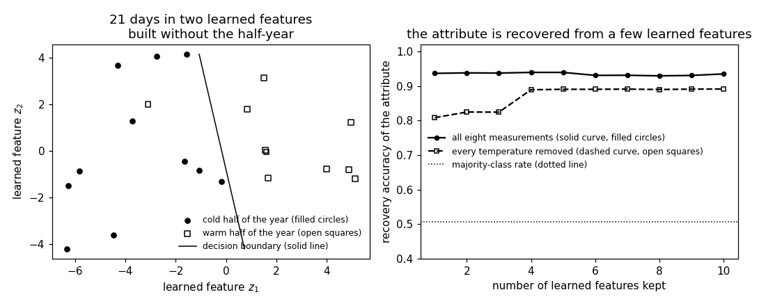
[B-plot]      Preview: the twenty-one drawn days in the two learned
              features with the decision boundary, and the accuracy
              against the number of learned features kept.

Outputs
-------
sensattr_weather.csv     : date and the eight measurements, 366 days of 2024
sensattr_points_plot.csv : z1, z2, s of the 21 days drawn in the entry's
                           Fig. 1(a) (every 18th day in calendar order)
sensattr_boundary.csv    : the two endpoints of the decision boundary drawn
                           in Fig. 1(a)
sensattr_accuracy.csv    : number of learned features, recovery accuracy
                           with all eight measurements and with every
                           temperature measurement removed
sensattr.png             : matplotlib preview (checking only)
"""

# /// script
# requires-python = ">=3.10"
# dependencies = ["matplotlib==3.10.7", "numpy==2.3.4"]
# ///

import json
import urllib.request
from pathlib import Path

import numpy as np
import matplotlib

matplotlib.use("Agg")
import matplotlib.pyplot as plt

OUT_DIR = Path(__file__).parent

report = []                         # collects (check name, pass/fail) pairs


def check(name, ok):                # records and prints one verification
    report.append((name, bool(ok)))
    print(f"  [{'ok' if ok else 'FAIL'}] {name}")
Installed 11 packages in 60ms
Download the eight daily measurements at Krems for 2024 and write them to sensattr_weather.csv; check the count and one pinned value against the archive.
print("[B-fetch] eight daily measurements at Krems an der Donau, 2024")
PARAMS = ["tlmin", "tlmax", "tl_mittel", "rr", "so_h", "rf_mittel",
          "p_mittel", "vv_mittel"]
URL = ("https://dataset.api.hub.geosphere.at/v1/station/historical/"
       f"klima-v2-1d?parameters={','.join(PARAMS)}&station_ids=3805"
       "&start=2024-01-01&end=2024-12-31")
CSV = OUT_DIR / "sensattr_weather.csv"
try:
    with urllib.request.urlopen(URL, timeout=120) as resp:
        payload = json.load(resp)
    params = payload["features"][0]["properties"]["parameters"]
    stamps = [t[:10] for t in payload["timestamps"]]
    M = np.stack([np.array(params[p]["data"], dtype=float) for p in PARAMS], 1)
    M[:, 3] = np.maximum(M[:, 3], 0.0)      # -1 marks a trace of rain
    with open(CSV, "w") as fh:
        fh.write("date," + ",".join(PARAMS) + "\n")
        for day, row in zip(stamps, M):
            fh.write(day + "," + ",".join(f"{v:g}" for v in row) + "\n")
    print(f"    downloaded {len(stamps)} days")
except OSError as err:
    print(f"    download failed ({err}); reading the committed CSV")
    rows = [line.split(",") for line in
            CSV.read_text().strip().splitlines()[1:]]
    stamps = [row[0] for row in rows]
    M = np.array([[float(v) for v in row[1:]] for row in rows])

check("[B-fetch] 366 days with eight measurements for 2024",
      M.shape == (366, 8))
check("[B-fetch] the record matches the archive (Feb 1: -3.8 to 10.4 deg)",
      stamps[31] == "2024-02-01" and np.allclose(M[31, :2], [-3.8, 10.4]))
[B-fetch] eight daily measurements at Krems an der Donau, 2024
    downloaded 366 days
  [ok] [B-fetch] 366 days with eight measurements for 2024
  [ok] [B-fetch] the record matches the archive (Feb 1: -3.8 to 10.4 deg)
Build the 361 data points: forty raw features (five previous days times eight measurements) and the attribute s (cold half of the year), which is not a feature; scale every raw feature to zero sample mean and unit sample variance.
print("[B-attribute] 361 days, forty raw features, the attribute s")
LAG = 5
days = np.arange(LAG, len(M))                   # January 6 .. December 31
month = np.array([int(stamps[t][5:7]) for t in days])
s = ((month <= 3) | (month >= 10)).astype(int)  # 1: cold half of the year
t_pm = 2 * s - 1                                # the same attribute as +-1
m = len(days)
TEMPERATURE = [0, 1, 2]                         # tlmin, tlmax, tl_mittel
ALL_EIGHT = list(range(8))
NO_TEMPERATURE = [j for j in ALL_EIGHT if j not in TEMPERATURE]


def raw_features(columns):
    """The measurements of the five previous days, one row per day,
    each raw feature scaled to zero sample mean and unit sample variance."""
    raw = np.stack([M[day - LAG:day][:, columns].ravel() for day in days])
    return (raw - raw.mean(axis=0)) / raw.std(axis=0)


X = raw_features(ALL_EIGHT)
X_no_temp = raw_features(NO_TEMPERATURE)
majority = float(max(s.mean(), 1 - s.mean()))
check(f"[B-attribute] {m} days with {X.shape[1]} raw features each; "
      f"{int(s.sum())} of them lie in the cold half of the year, so the "
      f"majority-class rate is {majority:.3f}",
      (m, X.shape[1]) == (361, 40) and X_no_temp.shape[1] == 25)
check("[B-attribute] the attribute s is not among the raw features: no "
      "raw feature is a function of the half-year alone",
      min(X[s == 1, 0].min(), X[s == 0, 0].min()) < 0 <
      max(X[s == 1, 0].max(), X[s == 0, 0].max()))
check("[B-attribute] every scaled raw feature has zero sample mean and "
      "unit sample variance",
      np.allclose(X.mean(axis=0), 0.0) and np.allclose(X.var(axis=0), 1.0))
[B-attribute] 361 days, forty raw features, the attribute s
  [ok] [B-attribute] 361 days with 40 raw features each; 178 of them lie in the cold half of the year, so the majority-class rate is 0.507
  [ok] [B-attribute] the attribute s is not among the raw features: no raw feature is a function of the half-year alone
  [ok] [B-attribute] every scaled raw feature has zero sample mean and unit sample variance
Learn two features: the two eigenvectors of the sample covariance matrix with the largest eigenvalues.
print("[B-features] two learned features from the raw ones")


def learned_features(raw, nr_kept):
    """The nr_kept eigenvectors of the sample covariance matrix with the
    largest eigenvalues, applied to the raw features; also the eigenvalues."""
    cov = raw.T @ raw / len(raw)
    eigvals, eigvecs = np.linalg.eigh(cov)
    order = np.argsort(eigvals)[::-1]
    return raw @ eigvecs[:, order[:nr_kept]], eigvals[order]


Z, eigvals = learned_features(X, 2)
Z_no_temp, eigvals_no_temp = learned_features(X_no_temp, 2)
check(f"[B-features] the largest eigenvalue carries "
      f"{100 * eigvals[0] / eigvals.sum():.0f} percent of the sum of all "
      f"40 eigenvalues, the second {100 * eigvals[1] / eigvals.sum():.0f} "
      f"percent", eigvals[0] > eigvals[1] > eigvals[2])
check("[B-features] the two learned features have zero sample mean, so "
      "no learned feature encodes the half-year by an offset",
      np.allclose(Z.mean(axis=0), 0.0, atol=1e-9))
[B-features] two learned features from the raw ones
  [ok] [B-features] the largest eigenvalue carries 41 percent of the sum of all 40 eigenvalues, the second 9 percent
  [ok] [B-features] the two learned features have zero sample mean, so no learned feature encodes the half-year by an offset
A linear classifier learned by least squares on the two learned features predicts s on the days it was not learned from; the accuracy, averaged over twenty random halvings of the 361 days, against the majority-class rate, against the raw features, and for one to ten learned features. Repeated with every temperature measurement removed from the raw features.
print("[B-recover] recovery accuracy of a linear classifier on the "
      "learned features")
NR_SPLITS = 20


def halvings():
    """Twenty halvings of the days into a training and a test set."""
    for seed in range(NR_SPLITS):
        order = np.random.default_rng(seed).permutation(m)
        yield order[:m // 2], order[m // 2:]


def classifier(features, train):
    """A linear classifier learned by least squares on the training days,
    returned as its weight vector with the intercept last."""
    design = np.hstack([features, np.ones((len(features), 1))])
    return np.linalg.lstsq(design[train], t_pm[train], rcond=None)[0]


def recovery_accuracy(features):
    """The accuracy of that classifier on the days it was not learned
    from, averaged over the twenty halvings."""
    accs = []
    for train, test in halvings():
        weights = classifier(features, train)
        design = np.hstack([features, np.ones((len(features), 1))])
        accs.append(float((np.sign(design[test] @ weights)
                           == t_pm[test]).mean()))
    return float(np.mean(accs)), float(np.min(accs)), float(np.max(accs))


acc_two, lo_two, hi_two = recovery_accuracy(Z)
acc_raw = recovery_accuracy(X)[0]
acc_two_nt, lo_two_nt, hi_two_nt = recovery_accuracy(Z_no_temp)
acc_raw_nt = recovery_accuracy(X_no_temp)[0]
check(f"[B-recover] two learned features recover s with accuracy "
      f"{acc_two:.3f} (over the twenty halvings between {lo_two:.3f} and "
      f"{hi_two:.3f}), against the majority-class rate {majority:.3f}",
      acc_two > 0.9 > majority)
check(f"[B-recover] the forty raw features themselves give {acc_raw:.3f}, "
      f"so the two learned features keep what the raw ones carry about s",
      acc_two > acc_raw - 0.05)
check(f"[B-recover] with every temperature measurement removed, two "
      f"learned features still give {acc_two_nt:.3f} (between "
      f"{lo_two_nt:.3f} and {hi_two_nt:.3f}) and the 25 raw features "
      f"{acc_raw_nt:.3f}", acc_two_nt > 0.8)
curve = []
for nr_kept in range(1, 11):
    a_all = recovery_accuracy(learned_features(X, nr_kept)[0])[0]
    a_nt = recovery_accuracy(learned_features(X_no_temp, nr_kept)[0])[0]
    curve.append((nr_kept, a_all, a_nt))
    print(f"    {nr_kept:2d} learned features: {a_all:.3f} with all eight "
          f"measurements, {a_nt:.3f} with every temperature removed")
check("[B-recover] one single learned feature already recovers s with "
      f"accuracy {curve[0][1]:.3f}", curve[0][1] > 0.85)
check("[B-recover] the accuracy stays above the majority-class rate for "
      "every number of kept learned features",
      all(a > majority and b > majority for _, a, b in curve))
[B-recover] recovery accuracy of a linear classifier on the learned features
  [ok] [B-recover] two learned features recover s with accuracy 0.938 (over the twenty halvings between 0.917 and 0.967), against the majority-class rate 0.507
  [ok] [B-recover] the forty raw features themselves give 0.920, so the two learned features keep what the raw ones carry about s
  [ok] [B-recover] with every temperature measurement removed, two learned features still give 0.825 (between 0.773 and 0.878) and the 25 raw features 0.894
     1 learned features: 0.936 with all eight measurements, 0.808 with every temperature removed
     2 learned features: 0.938 with all eight measurements, 0.825 with every temperature removed
     3 learned features: 0.937 with all eight measurements, 0.824 with every temperature removed
     4 learned features: 0.939 with all eight measurements, 0.889 with every temperature removed
     5 learned features: 0.939 with all eight measurements, 0.890 with every temperature removed
     6 learned features: 0.931 with all eight measurements, 0.890 with every temperature removed
     7 learned features: 0.931 with all eight measurements, 0.891 with every temperature removed
     8 learned features: 0.929 with all eight measurements, 0.890 with every temperature removed
     9 learned features: 0.930 with all eight measurements, 0.891 with every temperature removed
    10 learned features: 0.935 with all eight measurements, 0.891 with every temperature removed
  [ok] [B-recover] one single learned feature already recovers s with accuracy 0.936
  [ok] [B-recover] the accuracy stays above the majority-class rate for every number of kept learned features
Projecting ten learned features onto the orthogonal complement of the classifier's direction and learning again there: the accuracy drops but stays above the majority-class rate.
print("[B-remove] the attribute after one direction is projected out")
Z_ten = learned_features(X, 10)[0]
train, test = next(iter(halvings()))
weights_ten = classifier(Z_ten, train)
direction = weights_ten[:-1] / np.linalg.norm(weights_ten[:-1])
Z_perp = Z_ten - np.outer(Z_ten @ direction, direction)
design = np.hstack([Z_ten, np.ones((m, 1))])
acc_before = float((np.sign(design[test] @ weights_ten) == t_pm[test]).mean())
weights_perp = classifier(Z_perp, train)
design_perp = np.hstack([Z_perp, np.ones((m, 1))])
acc_after = float((np.sign(design_perp[test] @ weights_perp)
                   == t_pm[test]).mean())
check("[B-remove] the projected learned features carry no component "
      "along the direction", np.allclose(Z_perp @ direction, 0.0, atol=1e-9))
check(f"[B-remove] ten learned features recover s with accuracy "
      f"{acc_before:.3f} on this halving; after the direction is projected "
      f"out, a new classifier still reaches {acc_after:.3f}, above the "
      f"majority-class rate {majority:.3f}",
      acc_before > acc_after > majority)
[B-remove] the attribute after one direction is projected out
  [ok] [B-remove] the projected learned features carry no component along the direction
  [ok] [B-remove] ten learned features recover s with accuracy 0.928 on this halving; after the direction is projected out, a new classifier still reaches 0.840, above the majority-class rate 0.507
Preview: the twenty-one drawn days in the two learned features with the decision boundary, and the accuracy against the number of learned features kept.
print("[B-plot] the days drawn in the figure, the boundary, and the preview")
drawn = np.arange(0, m, 18)                 # every 18th day, 21 days
with open(OUT_DIR / "sensattr_points_plot.csv", "w") as fh:
    fh.write("z1,z2,s\n")
    for i in drawn:
        fh.write(f"{Z[i, 0]:.3f},{Z[i, 1]:.3f},{s[i]}\n")
weights_two = classifier(Z, train)
z1_lo, z1_hi = float(Z[drawn, 0].min()), float(Z[drawn, 0].max())
z2_lo, z2_hi = float(Z[drawn, 1].min()), float(Z[drawn, 1].max())


def boundary_z2(z1):
    """The second learned feature on the decision boundary."""
    return -(weights_two[0] * z1 + weights_two[2]) / weights_two[1]


# the drawn segment of the boundary: the part of the line that stays
# inside the range of the drawn days in both learned features
on_line = np.linspace(z1_lo, z1_hi, 2001)
inside = on_line[(boundary_z2(on_line) >= z2_lo)
                 & (boundary_z2(on_line) <= z2_hi)]
ends = (float(inside[0]), float(inside[-1]))
with open(OUT_DIR / "sensattr_boundary.csv", "w") as fh:
    fh.write("z1,z2\n")
    for z1 in ends:
        fh.write(f"{z1:.3f},{boundary_z2(z1):.3f}\n")
with open(OUT_DIR / "sensattr_accuracy.csv", "w") as fh:
    fh.write("kept,acc_all,acc_notemp\n")
    for nr_kept, a_all, a_nt in curve:
        fh.write(f"{nr_kept},{a_all:.4f},{a_nt:.4f}\n")
drawn_right = float(np.mean(
    (np.sign(np.hstack([Z[drawn], np.ones((len(drawn), 1))]) @ weights_two)
     == t_pm[drawn])))
check(f"[B-plot] of the {len(drawn)} days drawn in the figure (every "
      f"18th day in calendar order), the boundary puts "
      f"{drawn_right * len(drawn):.0f} on the side of their own attribute "
      f"value", drawn_right >= 0.85)

fig, (ax1, ax2) = plt.subplots(1, 2, figsize=(10, 4))
cold, warm = s[drawn] == 1, s[drawn] == 0
ax1.scatter(Z[drawn][cold, 0], Z[drawn][cold, 1], marker="o", color="black",
            s=22, label="cold half of the year (filled circles)")
ax1.scatter(Z[drawn][warm, 0], Z[drawn][warm, 1], marker="s",
            facecolors="none", edgecolors="black", s=26,
            label="warm half of the year (open squares)")
ax1.plot(list(ends), [boundary_z2(ends[0]), boundary_z2(ends[1])], "k-",
         lw=1.0, label="decision boundary (solid line)")
ax1.set_xlabel("learned feature $z_1$")
ax1.set_ylabel("learned feature $z_2$")
ax1.set_title("21 days in two learned features\nbuilt without the half-year")
ax1.legend(frameon=False, fontsize=8)
kept = [c[0] for c in curve]
ax2.plot(kept, [c[1] for c in curve], "k-o", ms=4,
         label="all eight measurements (solid curve, filled circles)")
ax2.plot(kept, [c[2] for c in curve], "k--s", ms=4, mfc="none",
         label="every temperature removed (dashed curve, open squares)")
ax2.axhline(majority, color="black", ls=":", lw=1.0,
            label="majority-class rate (dotted line)")
ax2.set_ylim(0.4, 1.02)
ax2.set_xlabel("number of learned features kept")
ax2.set_ylabel("recovery accuracy of the attribute")
ax2.set_title("the attribute is recovered from a few learned features")
ax2.legend(frameon=False, fontsize=8, loc="center left")
fig.tight_layout()
fig.savefig(OUT_DIR / "sensattr.png", dpi=110)

print()
failed = [name for name, ok in report if not ok]
print(f"{len(report) - len(failed)}/{len(report)} checks passed"
      + (f"; FAILED: {failed}" if failed else ""))
if failed:
    raise SystemExit(1)
[B-plot] the days drawn in the figure, the boundary, and the preview
  [ok] [B-plot] of the 21 days drawn in the figure (every 18th day in calendar order), the boundary puts 20 on the side of their own attribute value

15/15 checks passed
B-plot writes when the script runs