# online learning
*Entry of the [Dictionary of Applied Machine Learning](https://dictionaryofml.org) (course edition), by Alexander Jung, Aalto University. CC BY 4.0. Updated 2026-10-29. [HTML](https://dictionaryofml.org/terms/onlinelearning.html) · [typeset PDF](https://dictionaryofml.org/terms/onlinelearning.pdf) · [LaTeX](https://dictionaryofml.org/terms/onlinelearning.tex) · [Python demo](https://dictionaryofml.org/terms/onlinelearning.py) · [notebook](https://dictionaryofml.org/terms/onlinelearning.ipynb)*
Math is LaTeX with the book's macros expanded, so no notation package is needed to read it.
## Abstract
Online learning refers to machine learning methods that continuously update the model parameters as new data points arrive over time. This contrasts with offline methods such as linear regression, which solve empirical risk minimization once over a fixed training set. The updates are based on some form of feedback: examples are an entire loss function determined by the new data point, or a reward signal. Online gradient descent uses an entire loss function as feedback; bandit and reinforcement learning methods replace the unavailable gradient by an estimate from the feedback. The figure of merit is the regret: the accumulated loss minus that of fixed model parameters chosen in hindsight. A method is successful if its regret per round vanishes as the number of rounds grows.
## Definition
A weather station reports one temperature reading per hour, and a forecast for the next hour must be issued before that reading arrives. An offline method such as linear regression first collects readings into a training set and trains a model on it once. It then forecasts with the learned model parameters, which stay fixed from then on: while it collects, it issues no forecast, and after it has trained, it no longer learns. An online learning method instead adapts its model parameters every time a new reading arrives; Fig. 1 shows both on three days of readings.
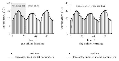
*Figure 1: Offline and online learning of a temperature forecaster on three days of hourly readings at Krems an der Donau (stems), both forecasting each hour from the readings of the three previous hours. (a) An offline method collects the readings of the first day into a training set, trains a linear regression forecaster on them once, and forecasts the next two days with the learned model parameters $\widehat{{\mathbf w}}$ held fixed; during the first day it issues no forecast. (b) An online method starts from ${\mathbf w}^{(1)} = \mathbf{0}$ at hour $0$, issues a forecast with its current model parameters ${\mathbf w}^{(t)}$ at every hour, and updates them as soon as the reading arrives; its first forecasts are far off, and within the first day it tracks the readings. Data generated by pythondemos/onlinelearning.py*
Online learning proceeds in rounds: in each round, a machine learning method commits to model parameters, receives a feedback signal from its environment, and updates (Cesa-Bianchi and Lugosi, 2006; Hazan, 2022, Sect. 1.1; Shalev-Shwartz, 2012). The updates are based on some form of feedback. For the weather station, the feedback is the new data point itself. Any new temperature reading allows to compute the squared error loss against the current model parameters, and the loss can be evaluated for any possible choice of the model parameters. The feedback is therefore an entire loss function ${\mathbf w} \mapsto L\left({\mathbf z}^{(t)},{\mathbf w} \right)$ (Hazan, 2022, Sect. 1.1). Online gradient descent is the online learning method for feedback by an entire loss function: it updates the model parameters by a gradient step on that loss function (Zinkevich, 2003).
Some online learning applications provide only a single loss or reward value as feedback, called bandit feedback in contrast to full information (Fig. 2). For example, a clinic that gives one of several treatments observes the outcome of that treatment alone, which is a multiarmed bandit (Lattimore and Szepesvári, 2020, Ch. 1). A thermostat whose heating decision changes the temperature it faces in the next hour receives a reward together with a new state, which is reinforcement learning (Sutton and Barto, 2018, Ch. 3).
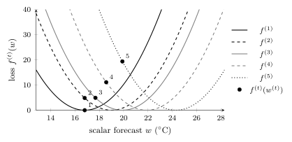
*Figure 2: The loss functions of five consecutive hours of the temperature stream in one plane ($f^{(1)}$ solid black, $f^{(2)}$ dashed black, $f^{(3)}$ solid gray, $f^{(4)}$ dashed gray, and $f^{(5)}$ dotted black curve), for the scalar forecaster $w$ and the squared error loss $f^{(t)}(w) = (y^{(t)} - w)^{2}$, which is smallest at the reading $y^{(t)}$ of hour $t$. With full information, the whole curve $f^{(t)}$ is revealed at hour $t$. With bandit feedback, only its value at the committed forecast $w^{(t)}$ is revealed (dots, labeled by $t$); here the forecasts are the iterates of online gradient descent, each moved toward the newest reading by a fixed fraction of the distance. Data generated by pythondemos/onlinelearning.py*
Consider model parameters ${\mathbf w}$ from a convex closed set $\mathcal{W} \subseteq \mathbb{R}^{d}$, the parameter space, and rounds at consecutive time instants $t = 1, 2, \ldots$. At time $t$, the environment fixes a function $f^{(t)}: \mathcal{W} \to \mathbb{R}$, and the current model parameters ${\mathbf w}^{(t)}$ incur the loss $f^{(t)}({\mathbf w}^{(t)})$. Only then is a feedback signal $r^{(t)}$ about $f^{(t)}$ revealed. The feedback signal is written $r^{(t)}$, in the reward notation of reinforcement learning, although with full information it is a data point and with bandit feedback a loss value. Three kinds of feedback occur.
With full information, the data point ${\mathbf z}^{(t)}$ is revealed, and it determines $f^{(t)}({\mathbf w}) = L\left({\mathbf z}^{(t)},{\mathbf w} \right)$ for every ${\mathbf w} \in \mathcal{W}$. On the temperature stream, the data point ${\mathbf z}^{(t)} = ({\mathbf x}^{(t)}, y^{(t)})$ has as features, collected in the feature vector ${\mathbf x}^{(t)}$, the readings of the previous hours, and as label the reading of hour $t$. Its loss function $f^{(t)}$ is the squared error loss of the forecast $h^{({\mathbf w})}({\mathbf x}^{(t)})$.
With bandit feedback, only the value $f^{(t)}({\mathbf w}^{(t)})$ is revealed. In a multiarmed bandit with $A$ actions, the model parameters ${\mathbf w}^{(t)} \in \Delta^{A-1}$ form the probability mass function from which the action $a^{(t)}$ is drawn. The environment fixes a loss vector $\boldsymbol{\ell}^{(t)} \in [0,1]^{A}$, whose entry $\ell^{(t)}_{a}$ is the loss of action $a$ in round $t$, so the expected loss of the draw is $f^{(t)}({\mathbf w}) = \langle \boldsymbol{\ell}^{(t)}, {\mathbf w} \rangle$. The clinic observes the single entry $\ell^{(t)}_{a^{(t)}}$, the loss of the action drawn, and no other entry.
With reinforcement learning feedback, the immediate reward $r(s^{(t)}, a^{(t)})$ of the action taken and the next state $s^{(t+1)}$ of a Markov decision process are revealed. The loss $f^{(t)}({\mathbf w})$ is the negative expected reward of the policy with model parameters ${\mathbf w}$ in the state $s^{(t)}$. That state depends on the actions of the earlier rounds, so the environment's losses depend on the method's own past.
The method then updates the model parameters using the feedback,
\begin{equation}
\tag{1}
{\mathbf w}^{(t+1)} :=
\mathcal{F}^{(t)}\big({\mathbf w}^{(t)}, r^{(t)}\big)
\text{,}
\end{equation}
with an update operator $\mathcal{F}^{(t)}$ specific to the method, the counterpart of the operator $\mathcal{F}$ of a fixed-point iteration (Fig. 3). The time index is also the iteration index: one update for any newly arriving data point. This contrasts with batch learning, which solves empirical risk minimization once over a fixed training set and then uses the learned hypothesis.
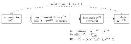
*Figure 3: One round of online learning. The method commits to the model parameters ${\mathbf w}^{(t)}$ before the environment fixes the loss $f^{(t)}$ of the round, incurs $f^{(t)}({\mathbf w}^{(t)})$, receives a feedback signal $r^{(t)}$, and updates to ${\mathbf w}^{(t+1)}$ for the next round. The feedback is the data point itself (full information, as in online gradient descent), the loss of the drawn action alone (bandit), or a reward and the next state (reinforcement learning)*
The update Eq. (1) at time $t$ applies an operator that depends on the feedback signal $r^{(t)}$. By contrast, gradient descent applies a fixed gradient step operator in every time step. An online learning method is therefore not a fixed-point iteration of one fixed operator. Instead, it concatenates operators that vary over the time steps. Unlike stochastic gradient descent, which uses one data point per step to approximate the gradient of one fixed objective function, an online learning method faces a different loss function in every round.
With full information, online gradient descent uses the gradient ${\mathbf g}^{(t)} := \nabla f^{(t)}({\mathbf w}^{(t)})$ in a projected gradient step. Online mirror descent replaces the Euclidean distance of the projection by a Bregman divergence, e.g., the Kullback–Leibler divergence on the probability simplex, which gives the Hedge update of the probability mass function over the actions (Hazan, 2022, Sect. 5.4). Follow-The-Regularized-Leader commits, in every round, to a minimizer of the accumulated loss of all rounds so far plus a regularizer (Hazan, 2022, Sect. 5.2).
With bandit feedback, the gradient of $f^{(t)}$ is not available, since only one entry of $\boldsymbol{\ell}^{(t)}$ is observed. Exp3 forms an unbiased estimate of $\boldsymbol{\ell}^{(t)}$ by dividing the observed entry by the probability of the drawn action, and applies the online mirror descent update to the estimate (Auer et al., 2002, Sect. 3).
With reinforcement learning feedback, Q-learning changes one entry of a table of action values, the entry of the state visited and the action taken. The entry moves by a fixed fraction of the difference between its target, the reward received plus the discounted largest value of the next state, and its current value. This is a stochastic step of the Bellman operator, a contraction (Bertsekas, 2007, Sect. 1.2), so Q-learning, unlike online gradient descent, does have a fixed point interpretation (Sutton and Barto, 2018, Sect. 6.5). Policy gradient methods instead estimate the gradient of the expected reward from the rewards collected along the visited states (Sutton and Barto, 2018, Ch. 13).
The figure of merit of an online learning method is not the decrease of an objective function along the iterates, which measures the progress of gradient descent: online learning has no fixed objective function. The loss function $f^{(t)}$ of round $t$ is evaluated once, around ${\mathbf w}^{(t)}$, and the next round brings a different loss function. Instead, an online learning method is evaluated by its regret.
The regret is the excessive accumulated loss compared to that of a fixed choice ${\mathbf w} \in \mathcal{W}$ of the model parameters. This fixed choice ${\mathbf w}$ is kept for all rounds $t = 1, \ldots, T$ and can be chosen after all losses are known. After $T$ rounds, the regret relative to ${\mathbf w} \in \mathcal{W}$ is
$$
\mathrm{Regret}_{T}({\mathbf w}) :=
\sum_{t=1}^{T} f^{(t)}({\mathbf w}^{(t)})
- \sum_{t=1}^{T} f^{(t)}({\mathbf w}) \text{.}
$$
In a multiarmed bandit, the fixed ${\mathbf w}$ of interest is the probability mass function concentrated on one action. The regret is then measured against the best single action in hindsight; in reinforcement learning, against the best fixed policy (Jaksch et al., 2010, Sect. 2).
No assumption is made on how the losses are generated: the regret is defined for every sequence $f^{(1)}, f^{(2)}, \ldots$, even one chosen by an opponent who has seen ${\mathbf w}^{(t)}$. An online learning method is successful if its regret per round, $\mathrm{Regret}_{T}({\mathbf w})/T$, vanishes as $T$ grows for every ${\mathbf w} \in \mathcal{W}$ (Shalev-Shwartz, 2012, Sect. 1.1).
**Regret bounds.** The rate at which the regret per round vanishes depends on the feedback. With full information and convex losses whose gradients have norm at most $G$ on a parameter space of diameter $D$, online gradient descent with the learning rate $\eta^{(t)} = D/(G\sqrt{t})$ has $\mathrm{Regret}_{T}({\mathbf w}) \le \tfrac{3}{2} DG\sqrt{T}$ (Hazan, 2022, Thm. 3.1). No online algorithm can guarantee a regret below a constant times $DG\sqrt{T}$ for every sequence: for each algorithm there is a sequence of losses on which its regret is at least that (Hazan, 2022, Thm. 3.2).
With bandit feedback over $A$ actions, the expected regret of Exp3 is at most $2\sqrt{(e-1) T A \ln A}$ (Auer et al., 2002, Cor. 3.2): observing one entry of $\boldsymbol{\ell}^{(t)}$ instead of all of them costs the factor $\sqrt{A}$. With reinforcement learning feedback in a Markov decision process with $S$ states and $A$ actions, the UCRL2 method has regret at most a constant times $S \sqrt{A T \ln T}$, the constant depending on how many steps it takes to reach any state from any other (Jaksch et al., 2010, Thm. 2). In each case the regret per round vanishes as $T$ grows.
Fig. 4 shows the regret per round of online gradient descent and of follow-the-leader, the Follow-The-Regularized-Leader method without its regularizer, which commits in every round to a minimizer of the accumulated loss so far, on a year of hourly temperature readings. For linear regression with the squared error loss, that minimizer is computed by the recursive least-squares update, which carries the least-squares solution from time $t - 1$ to time $t$ in closed form (Haykin, 2002).
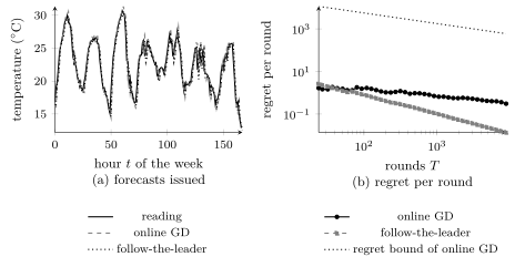
*Figure 4: Online learning of a temperature forecaster for Krems an der Donau in 2024. Each new temperature reading provides a new data point, with the readings of the three previous hours as features and the squared error loss. (a) One week of readings and the forecasts issued by online gradient descent and by follow-the-leader before each reading arrived. (b) The regret per round of both methods after $T$ rounds, relative to the model parameters that are best in hindsight over the same rounds, and the bound $DG/\sqrt{T}$ of online gradient descent. Data generated by pythondemos/onlinelearning.py*
Fig. 5 turns the same stream into a multiarmed bandit. The actions are five fixed forecasters, each a rule that needs no training. They forecast the previous reading, the reading of the same hour one day earlier, the mean of the three previous readings, the linear extrapolation of the two previous readings, and the mean of all readings of the year so far. The loss of an hour is the scaled absolute error of the forecaster used, and the regret is measured against the best single forecaster in hindsight.
With full information, all five errors are observed after each hour and Hedge updates the probability mass function; with bandit feedback, only the error of the forecaster used is observed and Exp3 updates the probability mass function from its estimate of the loss vector.
The regret of Hedge after $T$ rounds is at most $\sqrt{2 T \ln A}$ for losses in $[0,1]$, a weakening of the bound $\ln A / \eta + \eta T / 8$ of Cesa-Bianchi and Lugosi (2006, Thm. 2.2) at the learning rate $\eta = \sqrt{2 \ln A / T}$; for Exp3, the bound on the expected regret stated for bandit feedback applies with $A = 5$. Both regrets per round vanish, and the regret of Exp3 stays larger than that of Hedge, the increase in regret caused by bandit feedback.
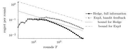
*Figure 5: The temperature stream as a multiarmed bandit with $A = 5$ fixed forecasters as actions. The regret per round after $T$ rounds against the best single forecaster in hindsight, for Hedge with full information (solid curve, filled circles) and for Exp3 with bandit feedback (dashed curve, filled squares), together with the bounds $\sqrt{2 \ln A / T}$ of Hedge (dotted curve) and $2\sqrt{(e-1) A \ln A / T}$ of Exp3 (dash-dotted curve). Data generated by pythondemos/onlinelearning.py*
**See also:** online gradient descent, online algorithm, regret, Hedge, Exp3, online mirror descent, mirror descent, Follow-The-Regularized-Leader, [stochastic gradient descent](https://dictionaryofml.org/terms/stochGD.html), [gradient descent](https://dictionaryofml.org/terms/gd.html), gradient step, [empirical risk minimization](https://dictionaryofml.org/terms/erm.html), risk, multiarmed bandit, [reinforcement learning](https://dictionaryofml.org/terms/reinforcementlearning.html), Markov decision process, Q-learning, batch learning, fixed-point iteration, [linear regression](https://dictionaryofml.org/terms/linreg.html).
## References
- Cesa-Bianchi and Lugosi (2006). Prediction, Learning, and Games. *Cambridge Univ. Press*.
- Hazan (2022). Introduction to Online Convex Optimization. *MIT Press*.
- Shalev-Shwartz (2012). Online Learning and Online Convex Optimization. *Foundations and Trends in Machine Learning*.
- Zinkevich (2003). Online Convex Programming and Generalized Infinitesimal Gradient Ascent. *Proc. 20th Int. Conf. Mach. Learn.*.
- Lattimore and Szepesvári (2020). Bandit Algorithms. *Cambridge University Press*.
- Sutton and Barto (2018). Reinforcement Learning: An Introduction. *MIT Press*.
- Auer et al. (2002). The Nonstochastic Multiarmed Bandit Problem. *SIAM J. Comput.*.
- Bertsekas (2007). Dynamic Programming and Optimal Control\textnormal{, vol. 2}. *Athena Scientific*.
- Jaksch et al. (2010). Near-optimal Regret Bounds for Reinforcement Learning. *Journal of Machine Learning Research*.
- Haykin (2002). Adaptive Filter Theory. *Prentice Hall*.
## Cite this entry
```bibtex
@misc{dictml_onlinelearning,
author = {Jung, Alexander},
editor = {Olioumtsevits, Konstantina and Schnoor, Ekkehard},
title = {online learning},
howpublished = {Dictionary of Applied Machine Learning (course edition)},
year = {2026},
doi = {10.5281/zenodo.21569296},
note = {ISBN 978-952-64-3013-3, CC BY 4.0, retrieved 2026-11-03},
url = {https://dictionaryofml.org/terms/onlinelearning.html}
}
```