B-reach writes when the script runsDictionary of Applied Machine Learning · learning rate
Numerical companion to the entry learning rate: it recomputes what the entry states and prints one line per check
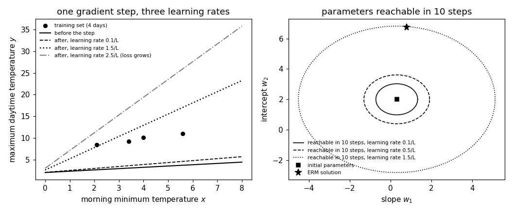
Shows what the learning rate of a gradient step does to the HYPOTHESIS MAP and to the set of model parameters that a fixed number of gradient steps can reach. One gradient step of GD on the average squared error loss of a linear model moves the fitted line by an amount proportional to the learning rate; a learning rate above 2/L makes the loss grow; and T steps with learning rate eta stay inside a ball around the initial parameters whose radius grows with eta. Self-contained (numpy and matplotlib only), fixed seed.
Run it without installing anything:uv run https://dictionaryofml.org/terms/learnrate.py
uv downloads this script and the pinned NumPy and Matplotlib it needs, then runs it; the script fetches any input file it uses. To keep the output files, download learnrate.py into a folder and run uv run learnrate.py there. With NumPy and Matplotlib already installed, python3 learnrate.py, from any directory — it writes its output files into the current directory. Fixed seeds, so the printed numbers reproduce exactly. Download learnrate.py · Notebook · Open in Colab
One cell per block of the script: the code, and what that code printed when it last ran here
"""
learnrate.py — numerical companion to the glossary entry 'learning rate'.

Purpose
-------
Shows what the learning rate of a gradient step does to the HYPOTHESIS
MAP and to the set of model parameters that a fixed number of gradient
steps can reach.  One gradient step of GD on the average squared error
loss of a linear model moves the fitted line by an amount proportional
to the learning rate; a learning rate above 2/L makes the loss grow; and
T steps with learning rate eta stay inside a ball around the initial
parameters whose radius grows with eta.  Self-contained (numpy and
matplotlib only), fixed seed.

Setup
-----
Training set: m = 4 consecutive days with feature x = morning minimum
temperature (degrees C) and label y = maximum daytime temperature
(degrees C); synthetic values drawn around y = 6.7 + 0.76 x.  Hypothesis
map h(x) = w1 x + w2, i.e. a linear model with the feature vector (x, 1).
Objective f(w) = average squared error loss on the training set, whose
Hessian is (2/m) X^T X with largest eigenvalue L.  Initial parameters
w = (0.3, 2.0), a poor line below the data.

Blocks
------
[B-data]  The training set, the initial hypothesis map and f at the
          initial parameters; L is reported.
[B-step]  One gradient step for three learning rates, 0.1/L, 1.5/L and
          2.5/L.  The change of the prediction at any x is eta times the
          product of the gradient with (x, 1), so the largest change of
          the line over the plotted range is exactly 15 times larger for
          1.5/L than for 0.1/L; the first two steps lower f, the third
          (above the threshold 2/L) raises it.
[B-reach] T = 10 gradient steps for the learning rates 0.1/L, 0.5/L and
          1.5/L.  Every iterate stays within the distance
          eta * sum_t ||grad f(w^(t))|| of the initial parameters, a
          radius that grows with eta; with 0.1/L the ERM solution lies
          outside that ball, with 1.5/L inside it.

Outputs
-------
learnrate_data.csv  : x, y of the 4 training days.
learnrate_lines.csv : x grid with h_before (initial line), h_small,
                      h_large, h_toolarge (after one step with 0.1/L,
                      1.5/L, 2.5/L).
learnrate_balls.csv : 91 points on each of the three circles of [B-reach]
                      (columns xs,ys / xm,ym / xl,yl) in the (w1, w2)
                      plane.
learnrate_reach.csv : one row per learning rate of [B-reach]: eta_over_L,
                      radius, w1_T, w2_T, plus the initial parameters and
                      the ERM solution as rows tagged in the first column.
learnrate.png       : matplotlib preview of the two figures (checking
                      only).
"""

import numpy as np
import matplotlib

matplotlib.use("Agg")
import matplotlib.pyplot as plt

from pathlib import Path

OUT_DIR = Path(__file__).parent

report = []


def check(name, ok):
    report.append((name, bool(ok)))
    print(f"  [{'ok' if ok else 'FAIL'}] {name}")


rng = np.random.default_rng(0)
The training set, the initial hypothesis map and f at the initial parameters; L is reported.
m = 4
x = np.array([2.1, 3.4, 4.0, 5.6])              # four consecutive days
y = 6.7 + 0.76 * x + 0.6 * rng.standard_normal(m)
X = np.c_[x, np.ones(m)]                        # feature vectors (x, 1)


def h(w, xs):
    return w[0] * xs + w[1]


def f(w):
    return float(np.mean((y - X @ w) ** 2))


def grad(w):
    return -(2.0 / m) * X.T @ (y - X @ w)


w0 = np.array([0.3, 2.0])
H = (2.0 / m) * X.T @ X
L = float(np.linalg.eigvalsh(H).max())
w_erm = np.linalg.lstsq(X, y, rcond=None)[0]
check(f"[B-data]  m={m} days, f(w0)={f(w0):.2f}, L={L:.1f}, "
      f"ERM solution w=({w_erm[0]:.2f}, {w_erm[1]:.2f})",
      f(w0) > 10.0 and L > 0)
[ok] [B-data] m=4 days, f(w0)=43.26, L=33.5, ERM solution w=(0.78, 6.75)
One gradient step for three learning rates, 0.1/L, 1.5/L and 2.5/L. The change of the prediction at any x is eta times the product of the gradient with (x, 1), so the largest change of the line over the plotted range is exactly 15 times larger for 1.5/L than for 0.1/L; the first two steps lower f, the third (above the threshold 2/L) raises it.
etas = {"small": 0.1 / L, "large": 1.5 / L, "toolarge": 2.5 / L}
g = grad(w0)
w_after = {k: w0 - e * g for k, e in etas.items()}
xg = np.linspace(0.0, 8.0, 81)
d = {k: np.abs(h(w_after[k], xg) - h(w0, xg)).max() for k in etas}
check(f"[B-step]  largest change of the line: {d['small']:.2f} (0.1/L) vs "
      f"{d['large']:.2f} (1.5/L), ratio {d['large'] / d['small']:.1f}",
      abs(d["large"] / d["small"] - 15.0) < 1e-6)
check(f"[B-step]  f: {f(w0):.2f} -> {f(w_after['small']):.2f} (0.1/L), "
      f"{f(w_after['large']):.2f} (1.5/L), {f(w_after['toolarge']):.2f} "
      f"(2.5/L, above 2/L: f grows)",
      f(w_after["small"]) < f(w0) and f(w_after["large"]) < f(w0)
      and f(w_after["toolarge"]) > f(w0))
  [ok] [B-step]  largest change of the line: 1.26 (0.1/L) vs 18.85 (1.5/L), ratio 15.0
  [ok] [B-step]  f: 43.26 -> 35.40 (0.1/L), 12.24 (1.5/L), 94.84 (2.5/L, above 2/L: f grows)
T = 10 gradient steps for the learning rates 0.1/L, 0.5/L and 1.5/L. Every iterate stays within the distance eta * sum_t ||grad f(w^(t))|| of the initial parameters, a radius that grows with eta; with 0.1/L the ERM solution lies outside that ball, with 1.5/L inside it.
T = 10
reach = {}
for tag, c in (("s", 0.1), ("m", 0.5), ("l", 1.5)):
    eta = c / L
    w = w0.copy(); path = 0.0
    for _ in range(T):
        gt = grad(w); path += eta * np.linalg.norm(gt); w = w - eta * gt
    reach[tag] = (c, path, w)
dist_erm = float(np.linalg.norm(w_erm - w0))
check(f"[B-reach] T={T}: radius {reach['s'][1]:.2f} (0.1/L), "
      f"{reach['m'][1]:.2f} (0.5/L), {reach['l'][1]:.2f} (1.5/L); "
      f"||w_ERM - w0|| = {dist_erm:.2f}",
      all(np.linalg.norm(reach[t][2] - w0) <= reach[t][1] + 1e-9
          for t in reach)
      and reach["s"][1] < dist_erm < reach["l"][1])

# ---------------------------------------------------------------- CSV
with open(OUT_DIR / "learnrate_data.csv", "w") as fh:
    fh.write("x,y\n")
    for a, b in zip(x, y):
        fh.write(f"{a:.3f},{b:.3f}\n")
with open(OUT_DIR / "learnrate_lines.csv", "w") as fh:
    fh.write("x,h_before,h_small,h_large,h_toolarge\n")
    for i, a in enumerate(xg):
        fh.write(f"{a:.3f},{h(w0, a):.3f},{h(w_after['small'], a):.3f},"
                 f"{h(w_after['large'], a):.3f},{h(w_after['toolarge'], a):.3f}\n")
ang = np.linspace(0.0, 2.0 * np.pi, 91)
with open(OUT_DIR / "learnrate_balls.csv", "w") as fh:
    fh.write("xs,ys,xm,ym,xl,yl\n")
    for a in ang:
        row = []
        for t in ("s", "m", "l"):
            r = reach[t][1]
            row += [f"{w0[0] + r * np.cos(a):.4f}", f"{w0[1] + r * np.sin(a):.4f}"]
        fh.write(",".join(row) + "\n")
with open(OUT_DIR / "learnrate_reach.csv", "w") as fh:
    fh.write("tag,eta_over_L,radius,w1,w2\n")
    fh.write(f"init,0,0,{w0[0]:.4f},{w0[1]:.4f}\n")
    fh.write(f"erm,0,0,{w_erm[0]:.4f},{w_erm[1]:.4f}\n")
    for t in ("s", "m", "l"):
        c, r, w = reach[t]
        fh.write(f"{t},{c},{r:.4f},{w[0]:.4f},{w[1]:.4f}\n")

# -------------------------------------------------------------- preview
fig, (ax, ax2) = plt.subplots(1, 2, figsize=(9.6, 4.0))
ax.plot(x, y, "ko", ms=5, label="training set (4 days)")
ax.plot(xg, h(w0, xg), "k-", lw=1.4, label="before the step")
ax.plot(xg, h(w_after["small"], xg), "k--", lw=1.2, label="after, learning rate 0.1/L")
ax.plot(xg, h(w_after["large"], xg), "k:", lw=1.6, label="after, learning rate 1.5/L")
ax.plot(xg, h(w_after["toolarge"], xg), "-.", color="0.5", lw=1.4,
        label="after, learning rate 2.5/L (loss grows)")
ax.set_xlabel("morning minimum temperature $x$")
ax.set_ylabel("maximum daytime temperature $y$")
ax.set_title("one gradient step, three learning rates")
ax.legend(frameon=False, fontsize=7)
for t, ls in (("s", "-"), ("m", "--"), ("l", ":")):
    c, r, w = reach[t]
    ax2.plot(w0[0] + r * np.cos(ang), w0[1] + r * np.sin(ang), "k", ls=ls, lw=1.1,
             label=f"reachable in {T} steps, learning rate {c}/L")
ax2.plot([w0[0]], [w0[1]], "ks", ms=5, label="initial parameters")
ax2.plot([w_erm[0]], [w_erm[1]], "k*", ms=9, label="ERM solution")
ax2.set_xlabel("slope $w_1$")
ax2.set_ylabel("intercept $w_2$")
ax2.set_title("parameters reachable in 10 steps")
ax2.legend(frameon=False, fontsize=7)
fig.tight_layout()
fig.savefig(OUT_DIR / "learnrate.png", dpi=110)

n_ok = sum(ok for _, ok in report)
print(f"\n{n_ok}/{len(report)} checks pass")
print(f"wrote {OUT_DIR / 'learnrate_data.csv'}, {OUT_DIR / 'learnrate_lines.csv'}, "
      f"{OUT_DIR / 'learnrate_balls.csv'}, {OUT_DIR / 'learnrate_reach.csv'}, "
      f"{OUT_DIR / 'learnrate.png'}")
if n_ok != len(report):
    raise SystemExit(1)
  [ok] [B-reach] T=10: radius 1.02 (0.1/L), 1.61 (0.5/L), 4.82 (1.5/L); ||w_ERM - w0|| = 4.77

4/4 checks pass
wrote /Users/junga1/dictionaryappliedml/pythondemos/learnrate_data.csv, /Users/junga1/dictionaryappliedml/pythondemos/learnrate_lines.csv, /Users/junga1/dictionaryappliedml/pythondemos/learnrate_balls.csv, /Users/junga1/dictionaryappliedml/pythondemos/learnrate_reach.csv, /Users/junga1/dictionaryappliedml/pythondemos/learnrate.png
B-reach writes when the script runs