B-preview writes when the script runsDictionary of Applied Machine Learning · kernel method
Numerical companion to the entry kernel method: it recomputes what the entry states and prints one line per check
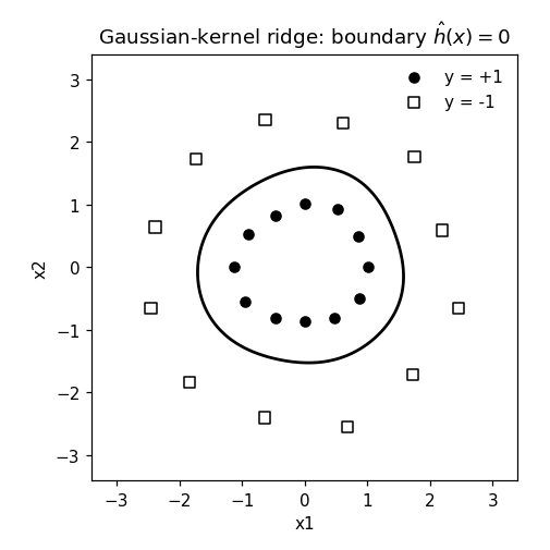
A two-ring binary trainset in R^2 that no linear classifier separates, on which a Gaussian-kernel method learns a perfect nonlinear decision boundary. The method is kernel ridge regression fit to labels y in {-1, +1}, with predictions taken as the sign of the fitted value — the construction known as regularized least-squares classification (Rifkin, Yeo & Poggio 2003). It is RERM over the RKHS H_k with the squared error loss,
Run it without installing anything:uv run https://dictionaryofml.org/terms/kernelmethod.py
uv downloads this script and the pinned NumPy and Matplotlib it needs, then runs it; the script fetches any input file it uses. To keep the output files, download kernelmethod.py into a folder and run uv run kernelmethod.py there. With NumPy and Matplotlib already installed, python3 kernelmethod.py, from any directory — it writes its output files into the current directory. Fixed seeds, so the printed numbers reproduce exactly. Download kernelmethod.py · Notebook · Open in Colab
One cell per block of the script: the code, and what that code printed when it last ran here
"""
kernelmethod.py — numerical companion to the glossary entry 'kernel method'.

Purpose
-------
A two-ring binary trainset in R^2 that no linear classifier separates, on
which a Gaussian-kernel method learns a perfect nonlinear decision boundary.
The method is kernel ridge regression fit to labels y in {-1, +1}, with
predictions taken as the sign of the fitted value — the construction known
as regularized least-squares classification (Rifkin, Yeo & Poggio 2003).
It is RERM over the RKHS H_k with the squared error loss,

    min_{h in H_k}  (1/m) sum_r (h(x^(r)) - y^(r))^2  +  alpha ||h||_{H_k}^2 ,

whose representer-theorem solution h_hat = sum_r beta_r k(x^(r), .) has the
closed-form expansion coefficients  beta_hat = (K + alpha m I)^{-1} y  with
Gram matrix K_rs = k(x^(r), x^(s)).  Self-contained (numpy/matplotlib only),
fixed seed.

Blocks
------
[B-data]   Two concentric rings (12 points each): class +1 on radius ~1.0,
           class -1 on radius ~2.5, radial noise 0.1, seed 0.
[B-linear] Baseline: least-squares linear classifier sign(w^T x + b) fit on
           the same trainset misclassifies about half the points — the
           dataset is far from linearly separable.
[B-kernel] Gaussian kernel k(x,x') = exp(-||x-x'||^2 / (2 sigma^2)) with
           sigma = 0.8, alpha = 1e-3: closed-form beta_hat, training
           accuracy 100%, boundary h_hat = 0 encircles the inner ring.
[B-opt]    Optimality check: K((K + alpha m I) beta_hat - y) = 0, the
           first-order optimality condition of the RERM objective in
           the coefficients, holds at beta_hat.
[B-norm]   The squared RKHS norm of the learned hypothesis, beta^T K beta.
[B-bnd]    The decision boundary h_hat = 0, as contour segments drawn
           onto the preview figure.
[B-csv]    The two CSVs the entry's pgfplots figure reads.
[B-preview] Data points and legend added to the preview figure; saved.

Outputs
-------
kernelmethod_points.csv   : the 24 data points, columns x1,x2,label,cls
                            (cls in {pos,neg}) for the entry's pgfplots
                            scatter.
kernelmethod_boundary.csv : polyline(s) of the learned decision boundary
                            h_hat(x) = 0, columns x1,x2; separate contour
                            segments are delimited by nan,nan rows
                            (pgfplots: unbounded coords=jump).
kernelmethod.png          : matplotlib preview of the figure (checking only).
"""

import numpy as np
import matplotlib

matplotlib.use("Agg")
import matplotlib.pyplot as plt

from pathlib import Path

OUT_DIR = Path(__file__).parent

report = []


def check(name, ok):
    report.append((name, bool(ok)))
    print(f"  [{'ok' if ok else 'FAIL'}] {name}")
kernel method demo (kernel ridge regression on +-1 labels, Gaussian kernel)
Two concentric rings (12 points each): class +1 on radius ~1.0, class -1 on radius ~2.5, radial noise 0.1, seed 0.
rng = np.random.default_rng(0)
m_per = 12
angles = np.linspace(0.0, 2.0 * np.pi, m_per, endpoint=False)

r_in = 1.0 + 0.1 * rng.standard_normal(m_per)
r_out = 2.5 + 0.1 * rng.standard_normal(m_per)
X_in = np.c_[r_in * np.cos(angles), r_in * np.sin(angles)]
X_out = np.c_[r_out * np.cos(angles + np.pi / m_per),
              r_out * np.sin(angles + np.pi / m_per)]

X = np.vstack([X_in, X_out])                    # (m, 2)
y = np.r_[np.ones(m_per), -np.ones(m_per)]      # +1 inner, -1 outer
m = len(y)

print("kernel method demo (kernel ridge regression on +-1 labels, "
      "Gaussian kernel)")
check("[B-data]   two rings, m = 24", m == 24 and set(y) == {1.0, -1.0})
[ok] [B-data] two rings, m = 24
Baseline: least-squares linear classifier sign(w^T x + b) fit on the same trainset misclassifies about half the points — the dataset is far from linearly separable.
A = np.c_[X, np.ones(m)]                        # [x1, x2, 1]
wb, *_ = np.linalg.lstsq(A, y, rcond=None)
acc_lin = np.mean(np.sign(A @ wb) == y)
check("[B-linear] linear least-squares baseline fails (acc <= 0.7)",
      acc_lin <= 0.7)
[ok] [B-linear] linear least-squares baseline fails (acc <= 0.7)
Gaussian kernel k(x,x') = exp(-||x-x'||^2 / (2 sigma^2)) with sigma = 0.8, alpha = 1e-3: closed-form beta_hat, training accuracy 100%, boundary h_hat = 0 encircles the inner ring.
SIGMA = 0.8
ALPHA = 1e-3


def gauss_kernel(P, Q):
    d2 = ((P[:, None, :] - Q[None, :, :]) ** 2).sum(-1)
    return np.exp(-d2 / (2.0 * SIGMA ** 2))


K = gauss_kernel(X, X)
beta = np.linalg.solve(K + ALPHA * m * np.eye(m), y)


def h_hat(P):
    """Representer expansion: h_hat(x) = sum_r beta_r k(x^(r), x)."""
    return gauss_kernel(P, X) @ beta


acc_ker = np.mean(np.sign(h_hat(X)) == y)
check("[B-kernel] kernel method separates the trainset (acc = 1.0)",
      acc_ker == 1.0)
[ok] [B-kernel] kernel method separates the trainset (acc = 1.0)
Optimality check: K((K + alpha m I) beta_hat - y) = 0, the first-order optimality condition of the RERM objective in the coefficients, holds at beta_hat.
opt_res = np.linalg.norm(K @ ((K + ALPHA * m * np.eye(m)) @ beta - y))
check("[B-opt]    first-order optimality condition holds at beta_hat",
      opt_res < 1e-8)
[ok] [B-opt] first-order optimality condition holds at beta_hat
The squared RKHS norm of the learned hypothesis, beta^T K beta.
rkhs_norm2 = float(beta @ K @ beta)
check("[B-norm]   RKHS norm ||h_hat||^2 positive and finite",
      0.0 < rkhs_norm2 < 1e6)
[ok] [B-norm] RKHS norm ||h_hat||^2 positive and finite
The decision boundary h_hat = 0, as contour segments drawn onto the preview figure.
# drawn directly onto the preview figure; [B-preview] finishes and saves it
G = 400
gx = np.linspace(-3.4, 3.4, G)
gy = np.linspace(-3.4, 3.4, G)
GX, GY = np.meshgrid(gx, gy)
HZ = h_hat(np.c_[GX.ravel(), GY.ravel()]).reshape(G, G)

fig, ax = plt.subplots(figsize=(4.6, 4.6))
cs = ax.contour(GX, GY, HZ, levels=[0.0], colors="k", linewidths=1.8)
segs = [s for s in cs.allsegs[0] if len(s) > 1]
check("[B-bnd]    boundary h_hat = 0 found", len(segs) >= 1)
  [ok] [B-bnd]    boundary h_hat = 0 found

linear baseline accuracy: 0.50 | kernel method accuracy: 1.00 | ||h_hat||^2_Hk = 12.43
6/6 checks pass
wrote /Users/junga1/dictionaryappliedml/pythondemos/kernelmethod_points.csv, /Users/junga1/dictionaryappliedml/pythondemos/kernelmethod_boundary.csv, /Users/junga1/dictionaryappliedml/pythondemos/kernelmethod.png
The two CSVs the entry's pgfplots figure reads.
with open(OUT_DIR / "kernelmethod_points.csv", "w") as f:
    f.write("x1,x2,label,cls\n")
    for xi, yi in zip(X, y):
        cls = "pos" if yi > 0 else "neg"
        f.write(f"{xi[0]:.4f},{xi[1]:.4f},{int(yi):+d},{cls}\n")

with open(OUT_DIR / "kernelmethod_boundary.csv", "w") as f:
    f.write("x1,x2\n")
    for i, s in enumerate(segs):
        if i:
            f.write("nan,nan\n")
        for p in s[::4]:                        # thin the polyline
            f.write(f"{p[0]:.4f},{p[1]:.4f}\n")
        f.write(f"{s[0][0]:.4f},{s[0][1]:.4f}\n")   # close the loop
Data points and legend added to the preview figure; saved.
ax.scatter(*X[y > 0].T, marker="o", c="k", s=35, label="y = +1")
ax.scatter(*X[y < 0].T, marker="s", facecolors="none", edgecolors="k",
           s=45, label="y = -1")
ax.set_xlabel("x1"), ax.set_ylabel("x2")
ax.set_aspect("equal")
ax.legend(frameon=False, loc="upper right")
ax.set_title("Gaussian-kernel ridge: boundary $\\hat{h}(x)=0$")
fig.tight_layout()
fig.savefig(OUT_DIR / "kernelmethod.png", dpi=110)

print(f"\nlinear baseline accuracy: {acc_lin:.2f}"
      f" | kernel method accuracy: {acc_ker:.2f}"
      f" | ||h_hat||^2_Hk = {rkhs_norm2:.2f}")
n_ok = sum(ok for _, ok in report)
print(f"{n_ok}/{len(report)} checks pass")
print(f"wrote {OUT_DIR / 'kernelmethod_points.csv'}, "
      f"{OUT_DIR / 'kernelmethod_boundary.csv'}, {OUT_DIR / 'kernelmethod.png'}")
if n_ok != len(report):
    raise SystemExit(1)
B-preview writes when the script runs