B-proj writes when the script runsDictionary of Applied Machine Learning · Hilbert space
Numerical companion to the entry Hilbert space: it recomputes what the entry states and prints one line per check
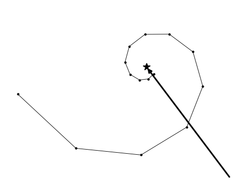
Backs the entry's completeness discussion and its two examples: it generates the Cauchy sequence shown in the entry's figure (converging to a limit that again belongs to the space), and it verifies that the expectation E{x x'} is an inner product on the finite-variance random variables of a common probability space, once random variables that are equal with probability one are identified. Self-contained (numpy only), fixed seeds.
Run it without installing anything:uv run https://dictionaryofml.org/terms/hilbertspace.py
uv downloads this script and the pinned NumPy and Matplotlib it needs, then runs it; the script fetches any input file it uses. To keep the output files, download hilbertspace.py into a folder and run uv run hilbertspace.py there. With NumPy and Matplotlib already installed, python3 hilbertspace.py, from any directory — it writes its output files into the current directory. Fixed seeds, so the printed numbers reproduce exactly. Download hilbertspace.py · Notebook · Open in Colab
One cell per block of the script: the code, and what that code printed when it last ran here
"""
hilbertspace.py — numerical companion to the glossary entry 'Hilbert space'.

Purpose
-------
Backs the entry's completeness discussion and its two examples: it
generates the Cauchy sequence shown in the entry's figure (converging
to a limit that again belongs to the space), and it verifies that the
expectation E{x x'} is an inner product on the finite-variance random
variables of a common probability space, once random variables that
are equal with probability one are identified.  Self-contained (numpy
only), fixed seeds.

Blocks
------
[B-cauchy]  The sequence w^(t) = w + 0.82^t * 2.3 * (cos(0.65 t + 2.7),
            sin(0.65 t + 2.7)) in R^2 is a Cauchy sequence: the
            diameter of the tail {w^(t) : t >= N} shrinks
            monotonically to 0.  Its limit is w = (-1.2, 1.6), an
            element of R^2 with finite induced norm — the limit stays
            in the space (completeness of the Euclidean space).
[B-rvspace] On a finite probability space (7 elements, one of
            them with probability zero), random variables are vectors in
            R^7 and the inner product <x, x'> = E{x x'} is the
            probability-weighted inner product of the vectors.  It is
            symmetric, bilinear and positive semi-definite; two random
            variables that differ only on the zero-probability element
            satisfy E{(x - x')^2} = 0 and have zero induced distance —
            they are identified (equal with probability one), and on
            the identified space the inner product is positive
            definite.
[B-proj]    Orthogonality principle in the Hilbert space of
            finite-variance random variables: the best linear
            approximation of y by a x (in the induced norm) has
            coefficient a* = E{x y} / E{x^2}, and the residual
            y - a* x is orthogonal to x, E{(y - a* x) x} = 0 —
            optimal estimation is orthogonal projection.

Outputs
-------
hilbertspace_cauchy.csv : points w^(1), ..., w^(14) of the Cauchy
                          sequence (columns x,y) for the entry's
                          pgfplots figure; the limit w = (-1.2, 1.6)
                          is drawn in TikZ directly.
hilbertspace.png        : matplotlib preview (checking only).
"""

import numpy as np                  # the only numerical dependency
import matplotlib

matplotlib.use("Agg")
import matplotlib.pyplot as plt

from pathlib import Path

OUT_DIR = Path(__file__).parent

report = []                         # collects (check name, pass/fail) pairs


def check(name, ok):                # records and prints one verification
    report.append((name, bool(ok)))
    print(f"  [{'ok' if ok else 'FAIL'}] {name}")
The sequence w^(t) = w + 0.82^t * 2.3 * (cos(0.65 t + 2.7), sin(0.65 t + 2.7)) in R^2 is a Cauchy sequence: the diameter of the tail {w^(t) : t >= N} shrinks monotonically to 0. Its limit is w = (-1.2, 1.6), an element of R^2 with finite induced norm — the limit stays in the space (completeness of the Euclidean space).
w_lim = np.array([-1.2, 1.6])       # the limit, an element of R^2
t = np.arange(1, 15)                # sequence indices t = 1, ..., 14
# a wide, slowly contracting spiral: the early elements sweep through the
# left half of the figure before closing in on the limit
pts = w_lim + (0.82 ** t)[:, None] * 2.3 * np.c_[
    np.cos(0.65 * t + 2.7), np.sin(0.65 * t + 2.7)]

# tail diameters diam{w^(t) : t >= N} shrink monotonically to zero
diams = [np.max([np.linalg.norm(p - q) for p in pts[N:] for q in pts[N:]])
         for N in range(0, 10)]
check("[B-cauchy]  tail diameters shrink monotonically (Cauchy property)",
      all(d1 > d2 for d1, d2 in zip(diams, diams[1:])) and diams[-1] < 0.5)
check("[B-cauchy]  the sequence converges to its limit in the space",
      np.linalg.norm(pts[-1] - w_lim) < 0.2
      and np.isfinite(np.sqrt(w_lim @ w_lim)))

with open(OUT_DIR / "hilbertspace_cauchy.csv", "w") as fh:
    fh.write("x,y\n")               # pgfplots table for the entry's figure
    for p in pts:
        fh.write(f"{p[0]:.4f},{p[1]:.4f}\n")
  [ok] [B-cauchy]  tail diameters shrink monotonically (Cauchy property)
  [ok] [B-cauchy]  the sequence converges to its limit in the space
On a finite probability space (7 elements, one of them with probability zero), random variables are vectors in R^7 and the inner product <x, x'> = E{x x'} is the probability-weighted inner product of the vectors. It is symmetric, bilinear and positive semi-definite; two random variables that differ only on the zero-probability element satisfy E{(x - x')^2} = 0 and have zero induced distance — they are identified (equal with probability one), and on the identified space the inner product is positive definite.
rng = np.random.default_rng(7)
K = 7                               # 7 elements, the last of probability zero
p = np.array([0.10, 0.15, 0.20, 0.25, 0.18, 0.12, 0.00])


def E(x):                           # expectation of a random variable
    return p @ x


def ip(x, y):                       # the entry's inner product <x, y> = E{x y}
    return E(x * y)


x, y, z = rng.standard_normal((3, K)) * 2.0          # three random variables
a, b = rng.standard_normal(2)                         # random coefficients

ok_sym = np.isclose(ip(x, y), ip(y, x))               # symmetry
ok_lin = np.isclose(ip(a * x + b * z, y),             # bilinearity
                    a * ip(x, y) + b * ip(z, y))
ok_psd = ip(x, x) >= 0                                # positive semi-definite
# E{x y} = probability-weighted inner product of the two vectors
ok_rep = np.isclose(ip(x, y), np.sum(p * x * y))
check("[B-rvspace] E{x y}: symmetric, bilinear, psd, weighted inner "
      "product", ok_sym and ok_lin and ok_psd and ok_rep)

xp = x.copy()
xp[-1] += 5.0                       # differs only on the probability-0 element
ok_ident = (np.isclose(ip(x - xp, x - xp), 0.0)       # E{(x - x')^2} = 0
            and np.isclose(np.sqrt(ip(x - xp, x - xp)), 0.0))
ok_pd = ip(x, x) > 0                # positive definite after identification
check("[B-rvspace] x and x' equal with probability one are identified",
      ok_ident and ok_pd)
  [ok] [B-rvspace] E{x y}: symmetric, bilinear, psd, weighted inner product
  [ok] [B-rvspace] x and x' equal with probability one are identified
Orthogonality principle in the Hilbert space of finite-variance random variables: the best linear approximation of y by a x (in the induced norm) has coefficient a* = E{x y} / E{x^2}, and the residual y - a* x is orthogonal to x, E{(y - a* x) x} = 0 — optimal estimation is orthogonal projection.
a_star = ip(x, y) / ip(x, x)        # best linear approximation of y by a x
resid = y - a_star * x              # estimation error
ok_orth = np.isclose(ip(resid, x), 0.0)               # orthogonality principle
# a* minimizes the induced norm of the residual over a grid of coefficients
grid = a_star + np.linspace(-1.0, 1.0, 201)
norms = [ip(y - a * x, y - a * x) for a in grid]
check("[B-proj]    residual of the best linear estimator is orthogonal "
      "to x", ok_orth and np.argmin(norms) == 100)

# ------------------------------------------------------------------ preview
fig, ax = plt.subplots(figsize=(4.2, 3.4))
ax.plot(pts[:, 0], pts[:, 1], "k.-", ms=4, lw=0.6)
ax.annotate("", xy=w_lim, xytext=(0, 0),
            arrowprops=dict(arrowstyle="-|>", lw=2))
ax.plot(*w_lim, "k*", ms=9)
ax.set_aspect("equal")
ax.set_xlabel("$w_1$"); ax.set_ylabel("$w_2$")
ax.set_title("Cauchy sequence and its limit in $\\mathbb{R}^2$")
fig.tight_layout()
fig.savefig(OUT_DIR / "hilbertspace.png", dpi=110)
[ok] [B-proj] residual of the best linear estimator is orthogonal to x
B-proj writes when the script runs# Kernel methods work in an RKHS: the Gaussian kernel's Gram matrix on
# any point set is symmetric psd (it defines an inner product on the
# span of kernel sections), and for f = sum_i a_i k(x_i, .) the
# reproducing property <f, k(x_j, .)> = f(x_j) holds — the inner product
# computed via the Gram matrix equals the pointwise evaluation computed
# directly from the kernel function.
rng_r = np.random.default_rng(3)
Pk = rng_r.normal(size=(8, 2))
kfun = lambda u, v: np.exp(-np.sum((u - v) ** 2) / 2.0)
K = np.array([[kfun(Pk[i], Pk[j]) for j in range(8)] for i in range(8)])
check("[B-rkhs] Gaussian Gram matrix is symmetric psd (an inner "
"product on kernel sections)",
np.allclose(K, K.T) and np.linalg.eigvalsh(K).min() > -1e-10)
a_coef = rng_r.normal(size=8)
inner_via_gram = K @ a_coef # <f, k(x_j,.)> = (K a)_j
f_pointwise = np.array([sum(a_coef[i] * kfun(Pk[i], Pk[j])
for i in range(8)) for j in range(8)])
check("[B-rkhs] reproducing property <f, k(x_j,.)> = f(x_j)",
np.allclose(inner_via_gram, f_pointwise))
n_ok = sum(ok for _, ok in report)
print(f"\n{n_ok}/{len(report)} checks pass")
print("wrote hilbertspace_cauchy.csv, pythondemos/hilbertspace.png")
if n_ok != len(report):
raise SystemExit(1)
  [ok] [B-rkhs]   Gaussian Gram matrix is symmetric psd (an inner product on kernel sections)
  [ok] [B-rkhs]   reproducing property <f, k(x_j,.)> = f(x_j)

7/7 checks pass
wrote hilbertspace_cauchy.csv, pythondemos/hilbertspace.png