B-plot writes when the script runsDictionary of Applied Machine Learning · Gaussian mixture model
Numerical companion to the entry Gaussian mixture model: it recomputes what the entry states and prints one line per check
Numerical companion to the glossary entry 'gmm' (Gaussian mixture model). A photograph of the Oetscher massif (assets/oetscher.jpg, the same photograph the 'kmeans' entry uses) is cut into square patches. Each patch is a data point whose feature vector holds two numbers, how green and how blue the patch is on average, so the covariance matrix of a component is a genuine matrix rather than a single number and each component shows as an ellipse in the plane.
Run it with python3 gmm.py, from any directory — it writes its output files into the current directory. Requires NumPy and Matplotlib only, and uses fixed seeds, so the printed numbers reproduce exactly. Download gmm.py · Notebook · Open in Colab
One cell per block of the script: the code, and what that code printed when it last ran here
"""A three-component GMM on the greenness and blueness of image patches:
meadow, foliage and sky, with graded membership where they meet.

Purpose
-------
Numerical companion to the glossary entry 'gmm' (Gaussian mixture
model).  A photograph of the Oetscher massif (assets/oetscher.jpg, the
same photograph the 'kmeans' entry uses) is cut into square patches.
Each patch is a data point whose feature vector holds two numbers, how
green and how blue the patch is on average, so the covariance matrix of
a component is a genuine matrix rather than a single number and each
component shows as an ellipse in the plane.

The demo checks the entry's claims: the cluster probabilities sum to
one; the three components are the sunlit meadow, the dark foliage and
the sky with the mountain; each covariance matrix is symmetric positive semi-definite;
the posterior distribution grades the membership of a patch in each
cluster instead of assigning it to exactly one; and the EM algorithm
reduces to k-means when the cluster probabilities are equal and every
covariance matrix is a shrinking multiple of the identity matrix.

Deterministic: the components are initialized by splitting the patches
into three equal parts ordered by blueness (no randomness).
Self-contained: numpy + matplotlib only.

Blocks
------
[B-patches]    Cut the photograph into 64x64 patches and measure how
               green and how blue each one is; check the patch count.
[B-em]         Fit the three-component GMM by the EM algorithm: E-step
               (posterior probability of each cluster index per patch),
               M-step (re-weighted cluster probabilities, means and
               covariance matrices).  Check that the cluster
               probabilities sum to one and that the fit stops changing.
[B-components] The three components are the sunlit meadow, the dark
               foliage, and the sky with the mountain.  Check each against the average color
               of its patches and against where they sit in the
               photograph, and check that each covariance matrix is
               symmetric positive semi-definite.
[B-soft]       Soft clustering: the posterior distribution grades
               membership.  Check that most patches are graded
               decisively and that the rest are shared between clusters.
[B-images]     The photograph with the patch grid drawn on it, the
               photograph at patch resolution, and one copy per
               cluster whose brightness is that cluster's posterior
               probability.  Because the posterior probabilities of a
               patch sum to one, the three copies add back up to the
               photograph.
[B-kmeans]     With equal cluster probabilities and covariance matrices
               that shrink to a multiple of the identity matrix, the
               posterior concentrates on the nearest mean and the EM
               update becomes the k-means update, so the algorithm
               reduces to k-means.  Check both.
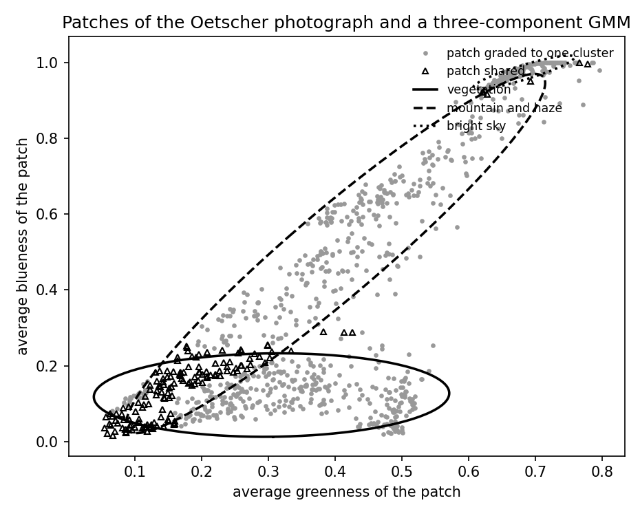
[B-plot]       Write the patch scatter and the three component ellipses
               for the entry's figure, plus the preview.

Outputs
-------
gmm_patches.csv  : green, blue -- every patch
gmm_points.csv   : x1, x2 -- the patches graded decisively
gmm_between.csv  : x1, x2 -- the patches shared between clusters
gmm_ellipse1.csv : x1, x2 -- contour of the meadow component
gmm_ellipse2.csv : x1, x2 -- contour of the foliage component
gmm_ellipse3.csv : x1, x2 -- contour of the sky component
gmm_oetscher_raster.png   : the photograph with the patch grid drawn on it
gmm_oetscher_original.png : the photograph at patch resolution
gmm_oetscher_vegetation.png : brightness = posterior of the vegetation cluster
gmm_oetscher_mountain.png   : brightness = posterior of the mountain cluster
gmm_oetscher_sky.png        : brightness = posterior of the sky cluster
gmm.png          : preview (checking only) -- the patches with the
                   three component ellipses drawn over them
"""

from pathlib import Path

import numpy as np
import matplotlib

matplotlib.use("Agg")
import matplotlib.pyplot as plt
from matplotlib.image import imread

OUT_DIR = Path(__file__).parent

report = []                         # collects (check name, pass/fail) pairs


def check(name, ok):                # records and prints one verification
    report.append((name, bool(ok)))
    print(f"  [{'ok' if ok else 'FAIL'}] {name}")
photograph cut into 27 x 36 = 972 patches of 128 x 128 pixels
Cut the photograph into 64x64 patches and measure how green and how blue each one is; check the patch count.
PATCH = 128
photo = imread(OUT_DIR.parent / "assets" / "oetscher.jpg") / 255.0
rows = photo.shape[0] // PATCH
cols = photo.shape[1] // PATCH
tiles = photo[:rows * PATCH, :cols * PATCH].reshape(
    rows, PATCH, cols, PATCH, 3).mean(axis=(1, 3))
rgb = tiles.reshape(-1, 3)
green = rgb[:, 1]                   # average greenness, on a 0 to 1 scale
blue = rgb[:, 2]                    # average blueness, on the same scale
X = np.column_stack([green, blue])
with open(OUT_DIR / "gmm_patches.csv", "w") as f:
    f.write("green,blue\n")
    for a, b in X:
        f.write(f"{a:.4f},{b:.4f}\n")
print(f"  photograph cut into {rows} x {cols} = {len(X)} patches "
      f"of {PATCH} x {PATCH} pixels")
check("[B-patches] every patch has a two-number feature vector",
      X.shape == (rows * cols, 2))
[ok] [B-patches] every patch has a two-number feature vector
Fit the three-component GMM by the EM algorithm: E-step (posterior probability of each cluster index per patch), M-step (re-weighted cluster probabilities, means and covariance matrices). Check that the cluster probabilities sum to one and that the fit stops changing.
NRCLUSTER = 3


def normal_pdf(A, mean, cov):
    """Density of the multivariate normal distribution at each row of A."""
    d = A.shape[1]
    diff = A - mean
    quad = np.einsum("ij,jk,ik->i", diff, np.linalg.inv(cov), diff)
    return np.exp(-0.5 * quad) / np.sqrt(((2.0 * np.pi) ** d)
                                         * np.linalg.det(cov))


def fit_quality(A, p, means, covs):
    """Negative log of the likelihood of the whole dataset."""
    mix = sum(p[c] * normal_pdf(A, means[c], covs[c]) for c in range(len(p)))
    return float(-np.log(mix).sum())


groups = np.array_split(np.argsort(X[:, 1]), NRCLUSTER)   # ordered by blueness
means = np.stack([X[g].mean(axis=0) for g in groups])
covs = np.stack([np.cov(X[g].T) for g in groups])
p = np.full(NRCLUSTER, 1.0 / NRCLUSTER)

trace = [fit_quality(X, p, means, covs)]
for _ in range(300):
    # E-step: posterior probability of each cluster index per patch
    joint = np.stack([p[c] * normal_pdf(X, means[c], covs[c])
                      for c in range(NRCLUSTER)])
    posterior = joint / joint.sum(axis=0)
    # M-step: re-weighted cluster probabilities, means, covariance matrices
    weight = posterior.sum(axis=1)
    p = weight / len(X)
    means = (posterior @ X) / weight[:, None]
    covs = np.stack([
        (posterior[c][:, None] * (X - means[c])).T @ (X - means[c]) / weight[c]
        for c in range(NRCLUSTER)])
    trace.append(fit_quality(X, p, means, covs))

order = np.argsort(means[:, 1])                  # greenest first, sky last
p, means, covs = p[order], means[order], covs[order]
posterior = posterior[order]
label = posterior.argmax(axis=0)

check("[B-em] the cluster probabilities sum to one",
      abs(p.sum() - 1.0) < 1e-12)
check("[B-em] the fit stops changing (last update tiny)",
      abs(trace[-1] - trace[-2]) < 1e-9)
  [ok] [B-em] the cluster probabilities sum to one
  [ok] [B-em] the fit stops changing (last update tiny)
  vegetation     probability 0.46, greenness +0.305, blueness +0.123, average color RGB [0.24 0.29 0.12], 15% of its patches in the upper half
  mountain and haze probability 0.39, greenness +0.401, blueness +0.496, average color RGB [0.26 0.43 0.54], 84% of its patches in the upper half
  bright sky     probability 0.15, greenness +0.683, blueness +0.974, average color RGB [0.36 0.68 0.97], 100% of its patches in the upper half
The three components are the sunlit meadow, the dark foliage, and the sky with the mountain. Check each against the average color of its patches and against where they sit in the photograph, and check that each covariance matrix is symmetric positive semi-definite.
NAMES = ("vegetation", "mountain and haze", "bright sky")
where = np.argwhere(np.ones((rows, cols), dtype=bool))    # (row, col) per patch
for c in range(NRCLUSTER):
    sel = label == c
    print(f"  {NAMES[c]:<14} probability {p[c]:.2f}, "
          f"greenness {means[c, 0]:+.3f}, blueness {means[c, 1]:+.3f}, "
          f"average color RGB {np.round(rgb[sel].mean(axis=0), 2)}, "
          f"{(where[sel][:, 0] < rows / 2).mean():.0%} of its patches in the "
          f"upper half")
check("[B-components] every average lies on the 0 to 1 scale",
      float(X.min()) >= 0.0 and float(X.max()) <= 1.0)
check("[B-components] the sky is the bluest component",
      means[2, 1] == means[:, 1].max())
check("[B-components] the sky sits in the upper half of the photograph",
      float((where[label == 2][:, 0] < rows / 2).mean()) > 0.8)
check("[B-components] the vegetation is the least blue and sits in the "
      "lower half", means[0, 1] == means[:, 1].min()
      and float((where[label == 0][:, 0] >= rows / 2).mean()) > 0.8)
check("[B-components] each covariance matrix is symmetric",
      all(np.allclose(c, c.T) for c in covs))
check("[B-components] each covariance matrix is positive semi-definite",
      all(np.linalg.eigvalsh(c).min() > 0 for c in covs))
  [ok] [B-components] every average lies on the 0 to 1 scale
  [ok] [B-components] the sky is the bluest component
  [ok] [B-components] the sky sits in the upper half of the photograph
  [ok] [B-components] the vegetation is the least blue and sits in the lower half
  [ok] [B-components] each covariance matrix is symmetric
  [ok] [B-components] each covariance matrix is positive semi-definite
  820 of 972 patches are graded above 0.8 for one cluster; 152 are shared
Soft clustering: the posterior distribution grades membership. Check that most patches are graded decisively and that the rest are shared between clusters.
top = posterior.max(axis=0)
shared = top < 0.8
print(f"  {int((~shared).sum())} of {len(X)} patches are graded above 0.8 "
      f"for one cluster; {int(shared.sum())} are shared")
check("[B-soft] the posterior distribution of each patch sums to one",
      np.allclose(posterior.sum(axis=0), 1.0))
check("[B-soft] most patches are graded decisively", (~shared).mean() > 0.8)
check("[B-soft] a shared patch is not assigned to exactly one cluster",
      bool(np.all(posterior[:, shared].max(axis=0) < 0.8)))
  [ok] [B-soft] the posterior distribution of each patch sums to one
  [ok] [B-soft] most patches are graded decisively
  [ok] [B-soft] a shared patch is not assigned to exactly one cluster
The photograph with the patch grid drawn on it, the photograph at patch resolution, and one copy per cluster whose brightness is that cluster's posterior probability. Because the posterior probabilities of a patch sum to one, the three copies add back up to the photograph.
def save_image(arr, name, zoom=6):
    """Write an RGB array as a PNG, enlarged so the patches stay visible."""
    img = np.clip(arr, 0.0, 1.0).repeat(zoom, axis=0).repeat(zoom, axis=1)
    plt.imsave(OUT_DIR / name, img)


# the photograph at full detail with the patch grid drawn on it, so
# the reader can see what one data point covers
SHRINK = 4
view = photo[:rows * PATCH, :cols * PATCH:, :][::SHRINK, ::SHRINK].copy()
cell = PATCH // SHRINK
view[::cell, :, :] = 1.0                       # horizontal rules
view[:, ::cell, :] = 1.0                       # vertical rules
view[-1, :, :] = 1.0
view[:, -1, :] = 1.0
save_image(view, "gmm_oetscher_raster.png", zoom=1)
check("[B-images] the raster has one cell per patch",
      view.shape[:2] == (rows * cell, cols * cell))

save_image(tiles, "gmm_oetscher_original.png")
COPIES = ("gmm_oetscher_vegetation.png", "gmm_oetscher_mountain.png",
          "gmm_oetscher_sky.png")
dimmed = [tiles * posterior[c].reshape(rows, cols, 1)
          for c in range(NRCLUSTER)]
for fname, arr in zip(COPIES, dimmed):
    save_image(arr, fname)
check("[B-images] one copy of the photograph per cluster",
      all((OUT_DIR / f).exists() for f in COPIES))
check("[B-images] the three copies add back up to the photograph",
      np.allclose(sum(dimmed), tiles))
  [ok] [B-images] the raster has one cell per patch
  [ok] [B-images] one copy of the photograph per cluster
  [ok] [B-images] the three copies add back up to the photograph
  variance 0.01: 85% of posteriors above 0.99, assignment agrees with k-means on 99.8% of patches
  variance 1e-05: 100% of posteriors above 0.99, assignment agrees with k-means on 99.8% of patches
With equal cluster probabilities and covariance matrices that shrink to a multiple of the identity matrix, the posterior concentrates on the nearest mean and the EM update becomes the k-means update, so the algorithm reduces to k-means. Check both.
def kmeans(A, cents):
    """Lloyd's algorithm from the given starting means."""
    while True:
        lab = ((A[:, None, :] - cents) ** 2).sum(axis=2).argmin(axis=1)
        new = np.stack([A[lab == c].mean(axis=0) for c in range(len(cents))])
        if np.allclose(new, cents):
            return lab, new
        cents = new


def spherical_em(A, cents, var):
    """EM with equal cluster probabilities and covariance matrices var*I."""
    post = None
    for _ in range(300):
        d2 = ((A[:, None, :] - cents) ** 2).sum(axis=2)
        logp = -d2 / (2.0 * var)
        post = np.exp(logp - logp.max(axis=1, keepdims=True))
        post /= post.sum(axis=1, keepdims=True)
        new = (post.T @ A) / post.sum(axis=0)[:, None]
        if np.allclose(new, cents):
            break
        cents = new
    return post.argmax(axis=1), cents, post


start = np.stack([X[g].mean(axis=0) for g in groups])
lab_km, cent_km = kmeans(X, start.copy())
for var in (1e-2, 1e-5):
    lab_em, cent_em, post = spherical_em(X, start.copy(), var)
    agree = float((lab_em == lab_km).mean())
    hard = float((post.max(axis=1) > 0.99).mean())
    print(f"  variance {var:g}: {hard:.0%} of posteriors above 0.99, "
          f"assignment agrees with k-means on {agree:.1%} of patches")
    if var == 1e-5:
        check("[B-kmeans] the posterior becomes a hard assignment", hard > 0.99)
        check("[B-kmeans] the assignment agrees with k-means", agree > 0.99)
        check("[B-kmeans] the means agree with the k-means centroids",
              np.abs(cent_em - cent_km).max() < 0.01)
  [ok] [B-kmeans] the posterior becomes a hard assignment
  [ok] [B-kmeans] the assignment agrees with k-means
  [ok] [B-kmeans] the means agree with the k-means centroids
Write the patch scatter and the three component ellipses for the entry's figure, plus the preview.
def ellipse(mean, cov, sigma=2.0, n=200):
    """Contour at `sigma` standard deviations of one component."""
    vals, vecs = np.linalg.eigh(cov)
    t = np.linspace(0.0, 2.0 * np.pi, n)
    circle = np.stack([np.cos(t), np.sin(t)])
    return (mean[:, None] + sigma * vecs @ (np.sqrt(vals)[:, None]
                                            * circle)).T


for name, sel in (("gmm_points.csv", ~shared), ("gmm_between.csv", shared)):
    with open(OUT_DIR / name, "w") as f:
        f.write("x1,x2\n")
        for a, b in X[sel]:
            f.write(f"{a:.4f},{b:.4f}\n")
for c, name in enumerate(("gmm_ellipse1.csv", "gmm_ellipse2.csv",
                          "gmm_ellipse3.csv")):
    with open(OUT_DIR / name, "w") as f:
        f.write("x1,x2\n")
        for a, b in ellipse(means[c], covs[c]):
            f.write(f"{a:.4f},{b:.4f}\n")

fig, ax = plt.subplots(figsize=(6.2, 5.0))
ax.plot(X[~shared, 0], X[~shared, 1], "o", color="0.6", markersize=2.2,
        linestyle="none", label="patch graded to one cluster")
ax.plot(X[shared, 0], X[shared, 1], "^", color="black", markersize=4,
        markerfacecolor="none", linestyle="none", label="patch shared")
for c, style in enumerate(("-", "--", ":")):
    e = ellipse(means[c], covs[c])
    ax.plot(e[:, 0], e[:, 1], color="black", linewidth=1.7, linestyle=style,
            label=NAMES[c])
ax.set_xlabel("average greenness of the patch")
ax.set_ylabel("average blueness of the patch")
ax.set_title("Patches of the Oetscher photograph and a three-component GMM")
ax.legend(frameon=False, loc="upper right", fontsize="small")
fig.tight_layout()
fig.savefig(OUT_DIR / "gmm.png", dpi=150)
plt.close(fig)
check("[B-plot] the three ellipses and the patch scatter were written",
      (OUT_DIR / "gmm_ellipse3.csv").exists()
      and (OUT_DIR / "gmm_points.csv").exists())

passed = sum(1 for _, ok in report if ok)
print(f"\n{passed}/{len(report)} checks pass")
  [ok] [B-plot] the three ellipses and the patch scatter were written

19/19 checks pass
B-plot writes when the script runs