P-stable writes when the script runsDictionary of Applied Machine Learning · generalization
Numerical companion to the entry generalization: it recomputes what the entry states and prints one line per check
One block per paragraph of the entry (marked [P...]): each block verifies numerically what the corresponding statement asserts. Self-contained (numpy/matplotlib only), fixed seed.
Run it without installing anything:uv run https://dictionaryofml.org/terms/generalization.py
uv downloads this script and the pinned NumPy and Matplotlib it needs, then runs it; the script fetches any input file it uses. To keep the output files, download generalization.py into a folder and run uv run generalization.py there. With NumPy and Matplotlib already installed, python3 generalization.py, from any directory — it writes its output files into the current directory. Fixed seeds, so the printed numbers reproduce exactly. Download generalization.py · Notebook · Open in Colab
One cell per block of the script: the code, and what that code printed when it last ran here
"""
generalization.py — numerical companion to the glossary entry
'generalization'.

One block per paragraph of the entry (marked [P...]): each block verifies
numerically what the corresponding statement asserts. Self-contained
(numpy/matplotlib only), fixed seed.

Blocks
------
[P-goal]     Generalization = accurate predictions on data points not
             used during training: a well-sized hypothesis space gives
             a test error close to its empirical risk.
[P-erm]      Low empirical risk does NOT guarantee generalization: a
             degree-12 polynomial drives the empirical risk near zero
             while its test error explodes; online (sequential) least
             squares faces the same gap.
[P-iid]      Under the iid assumption, the risk is the expected loss
             and the generalization gap is risk minus empirical risk:
             both estimated by Monte Carlo for the learned hypothesis.
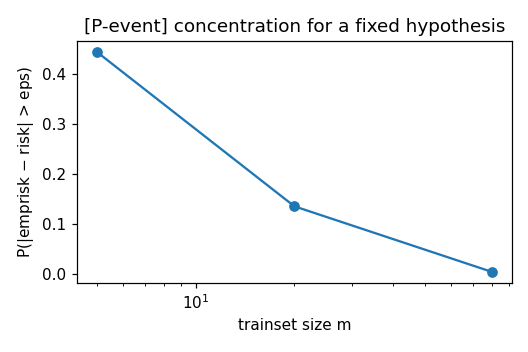
[P-event]    For a FIXED hypothesis h, the risk is deterministic while
             the empirical risk is an RV over trainset draws: its
             spread shrinks with m, so the probability of the event
             |emprisk - risk| > eps decays as m grows (concentration).
[P-stable]   The stability route: replacing one data point of the
             trainset changes the loss of the learned hypothesis only
             slightly on average, and the expected generalization gap
             is bounded by (in fact equals) that average change --
             verified by averaging over many trainset draws, with no
             reference to the size of the hypothesis space.

Outputs
-------
generalization.png : preview figure (checking only).

Data generated by pythondemos/generalization.py.
"""

import numpy as np
import matplotlib

matplotlib.use("Agg")
import matplotlib.pyplot as plt
from pathlib import Path

OUT_DIR = Path(__file__).parent

rng = np.random.default_rng(42)
report = []


def check(name, ok):
    report.append((name, bool(ok)))
    print(f"  [{'ok' if ok else 'FAIL'}] {name}")


f_true = lambda x: np.sin(2.0 * x)
def draw(m):
    x = rng.uniform(-1, 1, m)
    return x, f_true(x) + 0.2 * rng.normal(size=m)
Generalization = accurate predictions on data points not used during training: a well-sized hypothesis space gives a test error close to its empirical risk.
print("[P-goal] accuracy beyond the trainset")
xtr, ytr = draw(40)
xte, yte = draw(5000)
c3 = np.polyfit(xtr, ytr, 3)
tr3 = np.mean((ytr - np.polyval(c3, xtr)) ** 2)
te3 = np.mean((yte - np.polyval(c3, xte)) ** 2)
print(f"    degree 3: train {tr3:.3f}, test {te3:.3f}")
check("a well-sized model generalizes (test error close to the empirical risk)",
      te3 < 3 * tr3 and te3 < 0.08)
[P-goal] accuracy beyond the trainset
    degree 3: train 0.019, test 0.043
  [ok] a well-sized model generalizes (test error close to the empirical risk)
Low empirical risk does NOT guarantee generalization: a degree-12 polynomial drives the empirical risk near zero while its test error explodes; online (sequential) least squares faces the same gap.
print("[P-erm] low empirical risk does not guarantee generalization")
c12 = np.polyfit(xtr, ytr, 12)
tr12 = np.mean((ytr - np.polyval(c12, xtr)) ** 2)
te12 = np.mean((yte - np.polyval(c12, xte)) ** 2)
print(f"    degree 12: train {tr12:.4f}, test {te12:.2f}")
check("larger model: lower empirical risk", tr12 < tr3)
check("but much higher test error (no generalization guarantee)",
      te12 > 3 * te3)
# online learning faces the same challenge
w = np.zeros(13)
V = np.vander(xtr, 13)
for t in range(40):
    w += 0.05 * (ytr[t] - V[t] @ w) * V[t]
tr_ol = np.mean((ytr - V @ w) ** 2)
te_ol = np.mean((yte - np.vander(xte, 13) @ w) ** 2)
check("online learning shows a generalization gap too", te_ol > tr_ol)
[P-erm] low empirical risk does not guarantee generalization
    degree 12: train 0.0164, test 0.42
  [ok] larger model: lower empirical risk
  [ok] but much higher test error (no generalization guarantee)
  [ok] online learning shows a generalization gap too
Under the iid assumption, the risk is the expected loss and the generalization gap is risk minus empirical risk: both estimated by Monte Carlo for the learned hypothesis.
print("[P-iid] risk, empirical risk, and the generalization gap")
risk_hat = np.mean((yte - np.polyval(c3, xte)) ** 2)   # MC risk estimate
gap = risk_hat - tr3
print(f"    risk {risk_hat:.3f}, emprisk {tr3:.3f}, gap {gap:.3f}")
check("the generalization gap = risk - empirical risk is finite and "
      "computable under the iid model", np.isfinite(gap))
[P-iid] risk, empirical risk, and the generalization gap
    risk 0.043, emprisk 0.019, gap 0.024
  [ok] the generalization gap = risk - empirical risk is finite and computable under the iid model
For a FIXED hypothesis h, the risk is deterministic while the empirical risk is an RV over trainset draws: its spread shrinks with m, so the probability of the event |emprisk - risk| > eps decays as m grows (concentration).
print("[P-event] concentration of the empirical risk for fixed h")
h_fix = c3                                          # a FIXED hypothesis
risk_fix = np.mean((f_true(np.linspace(-1, 1, 10**5))
                    + 0.2 * rng.normal(size=10**5)
                    - np.polyval(h_fix, np.linspace(-1, 1, 10**5))) ** 2)
eps = 0.02
def event_prob(m, reps=600):
    hits = 0
    for _ in range(reps):
        x, y = draw(m)
        emp = np.mean((y - np.polyval(h_fix, x)) ** 2)
        hits += abs(emp - risk_fix) > eps
    return hits / reps
probs = [event_prob(m) for m in (5, 20, 80)]
print(f"    P(|emprisk - risk| > eps) at m = 5, 20, 80: "
      f"{probs[0]:.2f}, {probs[1]:.2f}, {probs[2]:.2f}")
check("the probability of a large deviation decays with m",
      probs[0] > probs[1] > probs[2])
check("at m = 80 the event is rare", probs[2] < 0.05)
[P-event] concentration of the empirical risk for fixed h
    P(|emprisk - risk| > eps) at m = 5, 20, 80: 0.45, 0.14, 0.00
  [ok] the probability of a large deviation decays with m
  [ok] at m = 80 the event is rare
The stability route: replacing one data point of the trainset changes the loss of the learned hypothesis only slightly on average, and the expected generalization gap is bounded by (in fact equals) that average change -- verified by averaging over many trainset draws, with no reference to the size of the hypothesis space.
print("[P-stable] stability bounds the expected generalization gap")
DEG_S, M_S, LAM, SIG = 3, 20, 0.1, 0.2
xg = np.linspace(-1, 1, 2001)                     # dense grid for the risk


def ridge_fit(x, y):
    V = np.vander(x, DEG_S + 1)
    return np.linalg.solve(V.T @ V + LAM * np.eye(DEG_S + 1), V.T @ y)


def risk_of(c):                                   # E[(y - h(x))^2], exact MC-free
    return float(np.mean((f_true(xg) - np.polyval(c, xg)) ** 2)) + SIG ** 2


gaps, changes = [], []
for _ in range(400):
    x, y = draw(M_S)
    c = ridge_fit(x, y)
    emp = float(np.mean((y - np.polyval(c, x)) ** 2))
    gaps.append(risk_of(c) - emp)
    i = int(rng.integers(M_S))                    # replace one data point
    xi, yi = x.copy(), y.copy()
    xi[i] = rng.uniform(-1, 1)
    yi[i] = f_true(xi[i]) + SIG * rng.normal()
    ci = ridge_fit(xi, yi)
    changes.append(float((y[i] - np.polyval(ci, x[i])) ** 2
                         - (y[i] - np.polyval(c, x[i])) ** 2))
lhs, rhs = np.mean(gaps), np.mean(changes)
print(f"    E[gap] {lhs:.4f}, average replace-one change of the loss {rhs:.4f}")
check("[P-stable] the expected gap matches the average replace-one change",
      abs(lhs - rhs) < 0.3 * abs(lhs) + 0.01)
check("[P-stable] the average absolute change bounds the expected gap",
      lhs <= np.mean(np.abs(changes)) + 0.01)

# ------------------------------------------------------------ preview
fig, ax = plt.subplots(figsize=(4.8, 3.2))
ax.semilogx([5, 20, 80], probs, "o-")
ax.set_xlabel("trainset size m")
ax.set_ylabel("P(|emprisk $-$ risk| > eps)")
ax.set_title("[P-event] concentration for a fixed hypothesis")
fig.tight_layout()
fig.savefig(OUT_DIR / "generalization.png", dpi=110)
print(f"\n{sum(ok for _, ok in report)}/{len(report)} checks passed")
assert all(ok for _, ok in report)
[P-stable] stability bounds the expected generalization gap
    E[gap] 0.0174, average replace-one change of the loss 0.0169
  [ok] [P-stable] the expected gap matches the average replace-one change
  [ok] [P-stable] the average absolute change bounds the expected gap

9/9 checks passed
P-stable writes when the script runs