B-plot writes when the script runsDictionary of Applied Machine Learning · feature space
Updated on 2026-11-19
Numerical companion to the entry feature space: it recomputes what the entry states and prints one line per check
Numerical companion to the glossary entry 'featurespace'. The 366 days of 2024 at Krems are the data points. Each day has a label, its maximum daytime temperature. The feature transformation decides which numbers describe a day, and its range is the feature space: the real line when a day is described by its morning minimum temperature alone, the plane when the maximum temperature of the previous day is added, and the finite set {1, ..., 12} when a day is described by its month.
Run it without installing anything:uv run https://dictionaryofml.org/terms/featurespace.py
uv downloads this script and the pinned NumPy and Matplotlib it needs, then runs it; the script fetches any input file it uses. To keep the output files, download featurespace.py into a folder and run uv run featurespace.py there. With NumPy and Matplotlib already installed, python3 featurespace.py, from any directory — it writes its output files into the current directory. Fixed seeds, so the printed numbers reproduce exactly. Download featurespace.py · Notebook · Open in Colab
Before running a downloaded copy, scan it: uvx bandit -q -t B102,B307,B602,B605 featurespace.py (B102,B307,B602,B605 are the exec, eval and shell checks of bandit) reports nothing: the script runs no shell command and evaluates no generated code.
One cell per block of the script: the code, and what that code printed when it last ran here
"""The feature space of the days of one year at Krems an der Donau: the
same days in three feature spaces, and the implicit feature space of a
kernel.

Purpose
-------
Numerical companion to the glossary entry 'featurespace'.  The 366 days
of 2024 at Krems are the data points.  Each day has a label, its maximum
daytime temperature.  The feature transformation decides which numbers
describe a day, and its range is the feature space: the real line when a
day is described by its morning minimum temperature alone, the plane
when the maximum temperature of the previous day is added, and the
finite set {1, ..., 12} when a day is described by its month.

The demo checks the entry's claims: the feature space is the set in
which the feature vectors live, and its geometry is what a method uses;
the same days have different nearest neighbors in different feature
spaces, and a linear hypothesis learned by least squares has a different
training error in each; on a finite feature space a hypothesis is a
table of values, every map on it is linear in the one-hot encoding, and
every other day of the same month is a nearest neighbor; the polynomial
kernel of degree two on the plane is the inner product in an explicit
six-dimensional feature space, while the Gaussian kernel has no
feature space of dimension below the number of data points.

Deterministic: no random numbers are used.  Self-contained: numpy +
matplotlib only; the GeoSphere download falls back to the committed CSV.

Blocks
------
[B-data]    Download the daily minimum and maximum temperature at Krems
            (GeoSphere station 3805) for 31 Dec 2023 to 31 Dec 2024 or
            read the committed copy; 366 days of 2024, each with the
            maximum temperature of the previous day.
[B-spaces]  Two feature transformations of the same days: the morning
            minimum alone (feature space R) and the pair morning
            minimum, previous day's maximum (feature space R^2).
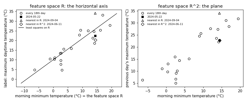
[B-nn]      The nearest neighbor of 22 May 2024 in R and in R^2 are
            different days with very different labels; 346 of the 366
            days change their nearest neighbor between the two spaces.
[B-linear]  A linear hypothesis learned by least squares in each space:
            training MSE 19.2 in R and 9.2 in R^2; the hypotheses on R
            are the hypotheses on R^2 that ignore the second feature.
[B-finite]  The finite feature space of the months: the hypothesis that
            minimizes the training MSE is the table of monthly means,
            MSE 17.0; least squares on the one-hot encoding learns the
            same table; under the discrete metric every other May day is
            a nearest neighbor of 22 May.
[B-kernel]  The polynomial kernel (1 + x^T x')^2 on R^2 equals the inner
            product of an explicit map into R^6, so its 366 x 366 matrix
            of kernel values has rank 6; for the Gaussian kernel with
            bandwidth 1 the matrix has rank 366.
[B-plot]    Every 18th day for the figure (21 of 366 days) plus 22 May
            and its two nearest neighbors, and the least-squares line
            on R.

Outputs
-------
featurespace_weather.csv     : date, tmin, tmax, prevtmax (committed copy).
featurespace_points_plot.csv : the drawn days with their role.
featurespace_line_plot.csv   : two points of the least-squares line on R.
featurespace.png             : matplotlib preview (checking only).
"""

# /// script
# requires-python = ">=3.10"
# dependencies = ["matplotlib==3.10.7", "numpy==2.3.4"]
# ///

import json
import urllib.request
from pathlib import Path

import numpy as np
import matplotlib

matplotlib.use("Agg")
import matplotlib.pyplot as plt

OUT_DIR = Path(__file__).parent
QUERY = "2024-05-22"

report = []


def check(name, ok):
    report.append((name, bool(ok)))
    print(f"  [{'ok' if ok else 'FAIL'}] {name}")
Download the daily minimum and maximum temperature at Krems (GeoSphere station 3805) for 31 Dec 2023 to 31 Dec 2024 or read the committed copy; 366 days of 2024, each with the maximum temperature of the previous day.
print("[B-data] daily minimum and maximum temperature at Krems, 2024")
URL = ("https://dataset.api.hub.geosphere.at/v1/station/historical/"
       "klima-v2-1d?parameters=tlmin,tlmax&station_ids=3805"
       "&start=2023-12-31&end=2024-12-31")
CSV = OUT_DIR / "featurespace_weather.csv"
try:
    with urllib.request.urlopen(URL, timeout=120) as resp:
        payload = json.load(resp)
    params = payload["features"][0]["properties"]["parameters"]
    raw = [(stamp[:10], lo, hi)
           for stamp, lo, hi in zip(payload["timestamps"],
                                    params["tlmin"]["data"],
                                    params["tlmax"]["data"])]
    if any(lo is None or hi is None for _, lo, hi in raw):
        raise OSError("a temperature is missing")
    # every day of 2024 with the maximum temperature of the previous day
    records = [(d, lo, hi, raw[i - 1][2])
               for i, (d, lo, hi) in enumerate(raw) if i > 0]
    with open(CSV, "w") as fh:
        fh.write("date,tmin,tmax,prevtmax\n")
        for d, lo, hi, pv in records:
            fh.write(f"{d},{lo},{hi},{pv}\n")
    print(f"    downloaded {len(raw)} days")
except OSError as err:
    print(f"    download failed ({err}); reading the committed CSV")
    rows = CSV.read_text().strip().splitlines()[1:]
    records = [(d, float(a), float(b), float(c))
               for d, a, b, c in (r.split(",") for r in rows)]

dates = [d for d, _, _, _ in records]
check("[B-data] 366 days of 2024, each with the previous day's maximum",
      len(records) == 366 and dates[0] == "2024-01-01"
      and dates[-1] == "2024-12-31")
tmin = np.array([lo for _, lo, _, _ in records])
tmax = np.array([hi for _, _, hi, _ in records])
prevtmax = np.array([pv for _, _, _, pv in records])
months = np.array([int(d[5:7]) for d in dates])
m = len(dates)
y = tmax                                   # the label of a day
[B-data] daily minimum and maximum temperature at Krems, 2024
    downloaded 367 days
  [ok] [B-data] 366 days of 2024, each with the previous day's maximum
Two feature transformations of the same days: the morning minimum alone (feature space R) and the pair morning minimum, previous day's maximum (feature space R^2).
print("[B-spaces] the same days in the feature spaces R and R^2")
X_A = tmin[:, None]                        # feature space R
X_B = np.column_stack([tmin, prevtmax])    # feature space R^2
check("[B-spaces] in R every day is a vector with d = 1 entry, in R^2 "
      "with d = 2 entries",
      X_A.shape == (m, 1) and X_B.shape == (m, 2))
check("[B-spaces] the first entry of a day's vector in R^2 is its vector "
      "in R: the two transformations agree on the shared feature",
      np.array_equal(X_B[:, :1], X_A))
check(f"[B-spaces] the {m} days occupy {len(np.unique(X_A))} points of R "
      f"and {len(np.unique(X_B, axis=0))} points of R^2",
      len(np.unique(X_A)) < m and len(np.unique(X_B, axis=0)) == m)


def nearest(X, q):
    """Index of the nearest other point and its Euclidean distance,
    plus the distance to the second-nearest (to confirm uniqueness)."""
    d = np.sqrt(np.sum((X - X[q]) ** 2, axis=1))
    d[q] = np.inf
    order = np.argsort(d)
    return int(order[0]), float(d[order[0]]), float(d[order[1]])
[B-spaces] the same days in the feature spaces R and R^2
  [ok] [B-spaces] in R every day is a vector with d = 1 entry, in R^2 with d = 2 entries
  [ok] [B-spaces] the first entry of a day's vector in R^2 is its vector in R: the two transformations agree on the shared feature
  [ok] [B-spaces] the 366 days occupy 196 points of R and 366 points of R^2
The nearest neighbor of 22 May 2024 in R and in R^2 are different days with very different labels; 346 of the 366 days change their nearest neighbor between the two spaces.
print(f"[B-nn] the nearest neighbor of {QUERY} in R and in R^2")
q = dates.index(QUERY)
nn_A, d_A, d_A2 = nearest(X_A, q)
nn_B, d_B, d_B2 = nearest(X_B, q)
check(f"[B-nn] {QUERY}: morning minimum {tmin[q]:.1f}, previous day's "
      f"maximum {prevtmax[q]:.1f}, label (maximum) {y[q]:.1f}",
      True)
check(f"[B-nn] nearest neighbor in R: {dates[nn_A]} (minimum "
      f"{tmin[nn_A]:.1f}, previous maximum {prevtmax[nn_A]:.1f}, label "
      f"{y[nn_A]:.1f}) at distance {d_A:.1f}, unique (next {d_A2:.1f})",
      d_A < d_A2)
check(f"[B-nn] nearest neighbor in R^2: {dates[nn_B]} (minimum "
      f"{tmin[nn_B]:.1f}, previous maximum {prevtmax[nn_B]:.1f}, label "
      f"{y[nn_B]:.1f}) at distance {d_B:.2f}, unique (next {d_B2:.2f})",
      d_B < d_B2)
check("[B-nn] the two nearest neighbors are different days",
      nn_A != nn_B)
check(f"[B-nn] the label of the neighbor in R misses the label of "
      f"{QUERY} by {abs(y[nn_A] - y[q]):.1f} degrees, the neighbor in R^2 "
      f"by {abs(y[nn_B] - y[q]):.1f}",
      abs(y[nn_A] - y[q]) > 10 > abs(y[nn_B] - y[q]))
changed = sum(nearest(X_A, i)[0] != nearest(X_B, i)[0] for i in range(m))
check(f"[B-nn] {changed} of the {m} days have a different nearest "
      f"neighbor in R than in R^2", changed > 0.9 * m)


def least_squares(X):
    """Linear hypothesis with intercept learned by least squares, and
    its training MSE."""
    Z = np.column_stack([np.ones(len(X)), X])
    w = np.linalg.lstsq(Z, y, rcond=None)[0]
    return w, float(np.mean((y - Z @ w) ** 2))
[B-nn] the nearest neighbor of 2024-05-22 in R and in R^2
  [ok] [B-nn] 2024-05-22: morning minimum 14.4, previous day's maximum 22.7, label (maximum) 22.4
  [ok] [B-nn] nearest neighbor in R: 2024-09-04 (minimum 14.4, previous maximum 34.0, label 34.1) at distance 0.0, unique (next 0.1)
  [ok] [B-nn] nearest neighbor in R^2: 2024-06-11 (minimum 14.5, previous maximum 22.7, label 20.2) at distance 0.10, unique (next 0.63)
  [ok] [B-nn] the two nearest neighbors are different days
  [ok] [B-nn] the label of the neighbor in R misses the label of 2024-05-22 by 11.7 degrees, the neighbor in R^2 by 2.2
  [ok] [B-nn] 346 of the 366 days have a different nearest neighbor in R than in R^2
A linear hypothesis learned by least squares in each space: training MSE 19.2 in R and 9.2 in R^2; the hypotheses on R are the hypotheses on R^2 that ignore the second feature.
print("[B-linear] least squares in R and in R^2")
w_A, mse_A = least_squares(X_A)
w_B, mse_B = least_squares(X_B)
check(f"[B-linear] on R: h(x) = {w_A[0]:.1f} + {w_A[1]:.2f} x, training "
      f"MSE {mse_A:.1f}", True)
check(f"[B-linear] on R^2: h(x) = {w_B[0]:.1f} + {w_B[1]:.2f} x_1 + "
      f"{w_B[2]:.2f} x_2, training MSE {mse_B:.1f}", True)
check("[B-linear] the hypothesis on R, read as a map on R^2 that ignores "
      "x_2, is a linear hypothesis on R^2 with the same training MSE",
      abs(least_squares(X_B)[1] - mse_B) < 1e-12
      and abs(np.mean((y - (w_A[0] + w_A[1] * X_B[:, 0])) ** 2) - mse_A)
      < 1e-12)
check("[B-linear] so the smaller feature space never gives a smaller "
      "training MSE: 19.2 > 9.2", mse_A > mse_B)
[B-linear] least squares in R and in R^2
  [ok] [B-linear] on R: h(x) = 10.0 + 1.10 x, training MSE 19.2
  [ok] [B-linear] on R^2: h(x) = 2.4 + 0.24 x_1 + 0.77 x_2, training MSE 9.2
  [ok] [B-linear] the hypothesis on R, read as a map on R^2 that ignores x_2, is a linear hypothesis on R^2 with the same training MSE
  [ok] [B-linear] so the smaller feature space never gives a smaller training MSE: 19.2 > 9.2
The finite feature space of the months: the hypothesis that minimizes the training MSE is the table of monthly means, MSE 17.0; least squares on the one-hot encoding learns the same table; under the discrete metric every other May day is a nearest neighbor of 22 May.
print("[B-finite] the month of a day as its feature: X = {1, ..., 12}")
table = np.array([y[months == k].mean() for k in range(1, 13)])
mse_M = float(np.mean((y - table[months - 1]) ** 2))
check("[B-finite] the hypothesis minimizing the training MSE is the table "
      f"of the 12 monthly means; its training MSE is {mse_M:.1f}",
      all(abs(np.mean((y - (table[months - 1] + delta * (months == k))) ** 2))
              >= mse_M - 1e-12
              for k in range(1, 13) for delta in (-0.5, 0.5)))
onehot = np.eye(12)[months - 1]
w_M = np.linalg.lstsq(onehot, y, rcond=None)[0]
check("[B-finite] least squares on the one-hot encoding learns the same "
      "table: every map on a finite feature space is linear in the "
      "one-hot vectors",
      np.allclose(w_M, table))
same_month = int(np.sum(months == months[q])) - 1
check(f"[B-finite] under the discrete metric all {same_month} other May "
      f"days are nearest neighbors of {QUERY}, at distance 0",
      same_month == 30)
check(f"[B-finite] training MSEs: {mse_A:.1f} (R), {mse_M:.1f} (months), "
      f"{mse_B:.1f} (R^2)", mse_B < mse_M < mse_A)
[B-finite] the month of a day as its feature: X = {1, ..., 12}
  [ok] [B-finite] the hypothesis minimizing the training MSE is the table of the 12 monthly means; its training MSE is 17.0
  [ok] [B-finite] least squares on the one-hot encoding learns the same table: every map on a finite feature space is linear in the one-hot vectors
  [ok] [B-finite] under the discrete metric all 30 other May days are nearest neighbors of 2024-05-22, at distance 0
  [ok] [B-finite] training MSEs: 19.2 (R), 17.0 (months), 9.2 (R^2)
The polynomial kernel (1 + x^T x')^2 on R^2 equals the inner product of an explicit map into R^6, so its 366 x 366 matrix of kernel values has rank 6; for the Gaussian kernel with bandwidth 1 the matrix has rank 366.
print("[B-kernel] polynomial and Gaussian kernel on the feature space R^2")
K_poly = (1.0 + X_B @ X_B.T) ** 2
phi = np.column_stack([np.ones(m), np.sqrt(2) * X_B[:, 0],
                       np.sqrt(2) * X_B[:, 1], X_B[:, 0] ** 2,
                       np.sqrt(2) * X_B[:, 0] * X_B[:, 1], X_B[:, 1] ** 2])
check("[B-kernel] (1 + x^T x')^2 equals the inner product of the explicit "
      "map into R^6 for every pair of days",
      np.allclose(K_poly, phi @ phi.T, rtol=1e-9, atol=1e-6))
rank_poly = np.linalg.matrix_rank(K_poly)
check(f"[B-kernel] the {m} x {m} matrix of polynomial kernel values has "
      f"rank {rank_poly} = dimension of that feature space", rank_poly == 6)
sq_dist = np.sum((X_B[:, None, :] - X_B[None, :, :]) ** 2, axis=-1)
K_gauss = np.exp(-sq_dist / 2.0)           # bandwidth 1 degree
rank_gauss = np.linalg.matrix_rank(K_gauss)
check(f"[B-kernel] the matrix of Gaussian kernel values (bandwidth 1) has "
      f"rank {rank_gauss}: no feature space of dimension below {m} "
      f"realizes it", rank_gauss == m)
check("[B-kernel] both matrices are positive semi-definite",
      np.linalg.eigvalsh(K_poly).min() > -1e-6
      and np.linalg.eigvalsh(K_gauss).min() > -1e-9)
[B-kernel] polynomial and Gaussian kernel on the feature space R^2
  [ok] [B-kernel] (1 + x^T x')^2 equals the inner product of the explicit map into R^6 for every pair of days
  [ok] [B-kernel] the 366 x 366 matrix of polynomial kernel values has rank 6 = dimension of that feature space
  [ok] [B-kernel] the matrix of Gaussian kernel values (bandwidth 1) has rank 366: no feature space of dimension below 366 realizes it
  [ok] [B-kernel] both matrices are positive semi-definite
Every 18th day for the figure (21 of 366 days) plus 22 May and its two nearest neighbors, and the least-squares line on R.
print("[B-plot] thinned scatter, the query day and its neighbors, the line")
idx = np.arange(0, m, 18)
roles = {q: 1, nn_A: 2, nn_B: 3}
drawn = sorted(set(idx) | set(roles))
with open(OUT_DIR / "featurespace_points_plot.csv", "w") as fh:
    fh.write("date,tmin,prevtmax,tmax,role\n")
    for i in drawn:
        fh.write(f"{dates[i]},{tmin[i]:.1f},{prevtmax[i]:.1f},{tmax[i]:.1f},"
                 f"{roles.get(i, 0)}\n")
check(f"[B-plot] every 18th day ({len(idx)} of the {m} days) plus "
      f"{QUERY} and its two nearest neighbors: {len(drawn)} days drawn",
      len(idx) == 21 and all(i in drawn for i in roles)
      and len(drawn) == len(set(idx) | set(roles)))
xs = np.array([tmin.min() - 1, tmin.max() + 1])
with open(OUT_DIR / "featurespace_line_plot.csv", "w") as fh:
    fh.write("tmin,yhat\n")
    for x in xs:
        fh.write(f"{x:.1f},{w_A[0] + w_A[1] * x:.3f}\n")

fig, (ax1, ax2) = plt.subplots(1, 2, figsize=(9.4, 3.9))
others = [i for i in drawn if roles.get(i, 0) == 0]
marks = ((others, "o", "none", "every 18th day"),
         ([q], "s", "black", f"{QUERY}"),
         ([nn_A], "^", "none", f"nearest in R: {dates[nn_A]}"),
         ([nn_B], "D", "none", f"nearest in R^2: {dates[nn_B]}"))
for sel, mk, face, lab in marks:
    ax1.scatter(tmin[sel], tmax[sel], marker=mk, facecolors=face,
                edgecolors="black", s=34, label=lab)
    ax2.scatter(tmin[sel], prevtmax[sel], marker=mk, facecolors=face,
                edgecolors="black", s=34, label=lab)
ax1.plot(xs, w_A[0] + w_A[1] * xs, "k-", lw=1,
         label="least squares on R")
ax1.set_xlabel("morning minimum temperature (°C) = the feature space R")
ax1.set_ylabel("label: maximum daytime temperature (°C)")
ax1.set_title("feature space R: the horizontal axis")
ax1.legend(frameon=False, fontsize=7)
ax2.plot([tmin[q], tmin[nn_B]], [prevtmax[q], prevtmax[nn_B]], "k--", lw=0.8)
ax2.set_xlabel("morning minimum temperature (°C)")
ax2.set_ylabel("previous day's maximum temperature (°C)")
ax2.set_title("feature space R^2: the plane")
ax2.legend(frameon=False, fontsize=7)
fig.tight_layout()
fig.savefig(OUT_DIR / "featurespace.png", dpi=110)

n_ok = sum(ok for _, ok in report)
print(f"\n{n_ok}/{len(report)} checks pass")
if n_ok != len(report):
    raise SystemExit(1)
[B-plot] thinned scatter, the query day and its neighbors, the line
  [ok] [B-plot] every 18th day (21 of the 366 days) plus 2024-05-22 and its two nearest neighbors: 23 days drawn

23/23 checks pass
B-plot writes when the script runs