B-faithful writes when the script runsDictionary of Applied Machine Learning · explanation
Numerical companion to the entry explanation: it recomputes what the entry states and prints one line per check
An explanation accompanies a prediction, and this demo produces both from real data. The data are hourly precipitation analyses of GeoSphere Austria (INCA, 1 km) over a 120 km box around Krems an der Donau for 8-17 September 2024, the days of storm Boris: 83 mm fell on Krems on 14 September alone (79 mm averaged over the 2 km cell holding the town). They are binned to a 60x60 grid of 2 km cells and committed as explanation_radar.csv, so this script needs no network. (The box was fetched once from the open data hub's grid endpoint, inca-v1-1h-1km, parameters=RR, output_format=netcdf, and binned 2x2 with Krems in the central cell.)
Run it without installing anything:uv run https://dictionaryofml.org/terms/explanation.py
uv downloads this script and the pinned NumPy and Matplotlib it needs, then runs it; the script fetches any input file it uses. To keep the output files, download explanation.py into a folder and run uv run explanation.py there. With NumPy and Matplotlib already installed, python3 explanation.py, from any directory — it writes its output files into the current directory. Fixed seeds, so the printed numbers reproduce exactly. Download explanation.py · Notebook · Open in Colab
One cell per block of the script: the code, and what that code printed when it last ran here
"""
explanation.py — numerical companion to the glossary entry 'explanation'.

Purpose
-------
An explanation accompanies a prediction, and this demo produces both from
real data.  The data are hourly precipitation analyses of GeoSphere
Austria (INCA, 1 km) over a 120 km box around Krems an der Donau for
8-17 September 2024, the days of storm Boris: 83 mm fell on Krems on
14 September alone (79 mm averaged over the 2 km cell holding the town).  They are binned to a 60x60 grid of 2 km cells and
committed as explanation_radar.csv, so this script needs no network.  (The
box was fetched once from the open data hub's grid endpoint,
inca-v1-1h-1km, parameters=RR, output_format=netcdf, and binned 2x2 with
Krems in the central cell.)

The prediction task is the one a reader can check against the sky: given
the precipitation over the box at hour t, will it rain at Krems at
hour t+2?  A small convolutional network is trained on the first days and
tested on the later ones.  Its explanation is a class activation map
obtained by Grad-CAM: how strongly the predicted score responds to each
convolutional activation map, averaged per map to one weight, then the
maps combined with these weights and rectified.  The CAM says which parts of the radar image the network used,
and the figure shows it by modulating the intensity of the radar image's
pixels: each cell's precipitation is scaled by its CAM score, so the cells
the network used stay visible and the rest fade.

Self-contained (numpy + matplotlib only), fixed seed.

Blocks
------
[B-data]  The committed radar frames, read back and checked against the
          storm they record: 79 mm falls on the Krems cell on 14 September, the
          wettest hour of the box exceeds 20 mm/h, and the 2-hour-ahead
          labels are close to balanced. The ten days are chosen so that
          rain falls in both halves of the chronological split -- with
          the storm alone, the held-out days are dry and the task there
          is trivially solved by answering "no rain".
[B-train] A convolutional network (one 3x3 layer, four channels, ReLU,
          global average pooling, linear head) fitted to the first 70% of
          the hours by lowering the logistic loss step by step.  Its accuracy on the
          held-out later hours beats the majority-class baseline.
[B-cam]   Grad-CAM for one held-out hour: the response of the score to
          each activation map, pooled to one weight per map, combined and
          rectified.  The map is written together with the
          radar image to explanation_frame.csv, which the entry's figure
          plots.
[B-text]  The same explanation as one sentence, read off the CAM: the
          radius around Krems that holds nine in ten of the cells the CAM
          scores highest (the tenth of the box the faithfulness test
          perturbs; the last tenth of them sit at the box's corner) and
          the compass direction of their centre of mass, checked against
          the precipitation actually recorded there.  The
          sentence is printed and drawn under the figure's panels.
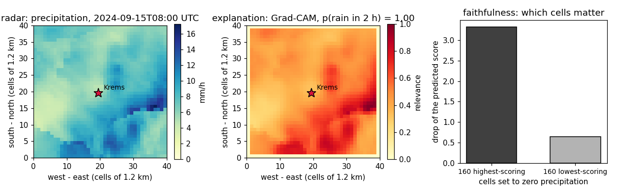
[B-faithful] The CAM is tested, not asserted.  Setting the precipitation
          to zero in the cells the CAM scores highest moves the predicted
          score much further than zeroing as many cells it scores lowest,
          and does so for the majority of held-out hours.

Outputs
-------
explanation_frame.csv : x, y, rr (mm/h), cam (0-1), rrcam (mm/h, the
                        precipitation scaled by the CAM) for the explained hour
explanation.png       : preview (checking only) — the radar image, the
                        radar image with its intensity modulated by the CAM,
                        the perturbation test, and the sentence under them
"""

import os

import numpy as np
import matplotlib

matplotlib.use("Agg")
import matplotlib.pyplot as plt

from pathlib import Path

OUT_DIR = Path(__file__).parent

report = []                         # collects (check name, pass/fail) pairs


def check(name, ok):                # records and prints one verification
    report.append((name, bool(ok)))
    print(f"  [{'ok' if ok else 'FAIL'}] {name}")


rng = np.random.default_rng(20240914)
N = 60                              # grid is N x N cells, 2 km each
KR, KC = 30, 30                     # cell holding Krems an der Donau
LEAD = 2                            # forecast lead time in hours
WET = 0.1                           # mm/h counting as rain
The committed radar frames, read back and checked against the storm they record: 79 mm falls on the Krems cell on 14 September, the wettest hour of the box exceeds 20 mm/h, and the 2-hour-ahead labels are close to balanced. The ten days are chosen so that rain falls in both halves of the chronological split -- with the storm alone, the held-out days are dry and the task there is trivially solved by answering "no rain".
# The committed radar file is an INPUT, unlike the CSVs the other demos
# generate, so it is read from beside this script rather than from the
# working directory: the demo then runs from anywhere, including the
# throwaway directory the site export uses (which carries an empty
# pythondemos/ so that OUTPUTS do not overwrite the committed ones).
RADAR = os.path.join(os.path.dirname(os.path.abspath(__file__)),
                     "explanation_radar.csv")
ncol = len(open(RADAR).readline().split(",")) - 2
if ncol != N * N:
    raise SystemExit(f"{RADAR} holds {ncol} cells per hour, this demo expects "
                     f"{N} x {N} = {N * N}: the committed grid and the script "
                     f"disagree")
raw = np.loadtxt(RADAR, delimiter=",", skiprows=1,
                 usecols=range(2, 2 + N * N))
stamps = [ln.split(",")[1] for ln in
          open(RADAR).read().splitlines()[1:]]
image = raw.reshape(-1, N, N) / 10.0                 # back to mm/h
krems = image[:, KR, KC]

daily = [krems[d * 24:(d + 1) * 24].sum() for d in range(10)]
check("[B-data] 14 September brings over 70 mm to the Krems cell (storm Boris)",
      max(daily) > 70.0)
check("[B-data] the wettest hour in the box exceeds 20 mm/h",
      image.max() > 20.0)

X = image[:-LEAD]                                     # input at hour t
y = (krems[LEAD:] > WET).astype(float)                # rain at Krems at t+2
check(f"[B-data] {len(y)} samples, {int(y.sum())} of them with rain ahead",
      len(y) == 238 and 0.35 < y.mean() < 0.65)

ntr = int(0.7 * len(y))
Xtr, ytr, Xte, yte = X[:ntr], y[:ntr], X[ntr:], y[ntr:]
check("[B-data] rain falls in both halves of the split, so neither is trivial",
      0.3 < ytr.mean() < 0.7 and 0.3 < yte.mean() < 0.7)
scale = Xtr.std()
Xtr, Xte = Xtr / scale, Xte / scale
print(f"  train {len(ytr)} hours ({stamps[0]} ..), test {len(yte)} hours "
      f"(.. {stamps[len(y) - 1]})")
  [ok] [B-data] 14 September brings over 70 mm to the Krems cell (storm Boris)
  [ok] [B-data] the wettest hour in the box exceeds 20 mm/h
  [ok] [B-data] 238 samples, 109 of them with rain ahead
  [ok] [B-data] rain falls in both halves of the split, so neither is trivial
  train 166 hours (2024-09-08T00:00 ..), test 72 hours (.. 2024-09-17T21:00)
  loss 1.191 -> 0.280, train acc 0.90, test acc 0.83, majority baseline 0.53
A convolutional network (one 3x3 layer, four channels, ReLU, global average pooling, linear head) fitted to the first 70% of the hours by lowering the logistic loss step by step. Its accuracy on the held-out later hours beats the majority-class baseline.
K, F = 4, 3                                           # channels, window size
M = N - F + 1                                         # activation map side


def to_grid(m):
    """Place an M x M activation map back on the N x N input grid.

    The convolution is valid, so activation-map cell (i, j) is computed from
    input cells i..i+F-1, and the map covers the input minus a one-cell
    border.  Padding it back into the centre keeps map and field aligned.
    Upsampling by repetition and cropping to [:N, :N] does NOT: it keeps
    the upper-left corner of a 2M x 2M array and shifts the explanation
    away from the weather it explains.
    """
    out = np.zeros((N, N))
    pad = (N - M) // 2
    out[pad:pad + M, pad:pad + M] = m
    return out


def forward(imgs, W, b, v, c):
    """Conv -> ReLU -> global average pool -> linear.  Returns (score, A)."""
    n = len(imgs)
    A = np.zeros((n, K, M, M))
    for i in range(F):
        for j in range(F):
            patch = imgs[:, i:i + M, j:j + M]         # (n, M, M)
            A += W[None, :, i, j, None, None] * patch[:, None]
    A = np.maximum(A + b[None, :, None, None], 0.0)   # (n, K, M, M)
    g = A.mean(axis=(2, 3))                           # (n, K)
    return g @ v + c, A


def backward(imgs, A, err, W, v):
    """How the mean logistic loss changes with W, b, v, c (for the update)."""
    n = len(imgs)
    g = A.mean(axis=(2, 3))
    gv, gc = g.T @ err / n, err.mean()
    dA = (err[:, None] @ v[None, :])[:, :, None, None] / (M * M)
    dA = np.repeat(np.repeat(dA, M, axis=2), M, axis=3) * (A > 0)
    gW = np.zeros_like(W)
    for i in range(F):
        for j in range(F):
            patch = imgs[:, i:i + M, j:j + M]
            gW[:, i, j] = np.einsum("nkxy,nxy->k", dA, patch) / n
    return gW, dA.sum(axis=(2, 3)).mean(axis=0), gv, gc


W = rng.normal(0, 0.5, (K, F, F))
b = np.zeros(K)
v = rng.normal(0, 0.5, K)
c = 0.0
lrate, losses = 0.5, []
for step in range(600):
    s, A = forward(Xtr, W, b, v, c)
    p = 1.0 / (1.0 + np.exp(-s))
    losses.append(-np.mean(ytr * np.log(p + 1e-9) + (1 - ytr) * np.log(1 - p + 1e-9)))
    gW, gb, gv, gc = backward(Xtr, A, p - ytr, W, v)
    W -= lrate * gW
    b -= lrate * gb
    v -= lrate * gv
    c -= lrate * gc

acc = lambda Xs, ys: float((( forward(Xs, W, b, v, c)[0] > 0) == (ys > 0.5)).mean())
base = max(yte.mean(), 1 - yte.mean())
print(f"  loss {losses[0]:.3f} -> {losses[-1]:.3f}, "
      f"train acc {acc(Xtr, ytr):.2f}, test acc {acc(Xte, yte):.2f}, "
      f"majority baseline {base:.2f}")
check("[B-train] the loss decreases", losses[-1] < 0.6 * losses[0])
check("[B-train] test accuracy beats the majority-class baseline",
      acc(Xte, yte) > base + 0.05)
  [ok] [B-train] the loss decreases
  [ok] [B-train] test accuracy beats the majority-class baseline
  explained hour 2024-09-15T08:00 UTC: predicted rain at Krems in 2 h with score 1.00; observed rain
Grad-CAM for one held-out hour: the response of the score to each activation map, pooled to one weight per map, combined and rectified. The map is written together with the radar image to explanation_frame.csv, which the entry's figure plots.
# The explained hour: the held-out hour with the highest predicted score,
# i.e. the one the network is most sure will bring rain to Krems.
ste, _ = forward(Xte, W, b, v, c)
pick = int(np.argmax(ste))
img = Xte[pick]
score, A = forward(img[None], W, b, v, c)
prob = float(1.0 / (1.0 + np.exp(-score[0])))

# Grad-CAM: d(score)/d(A) pooled per activation map gives one weight per map;
# the map is the rectified weighted sum of the activation maps.
dA = np.repeat(np.repeat((v[:, None, None] / (M * M))[None], M, axis=2),
               M, axis=3) * (A > 0)
alpha = dA[0].mean(axis=(1, 2))                       # one weight per map
cam = np.maximum((alpha[:, None, None] * A[0]).sum(axis=0), 0.0)
cam = cam / cam.max() if cam.max() > 0 else cam
cam_full = to_grid(cam)

hour = stamps[ntr + pick]
truth = "rain" if yte[pick] > 0.5 else "no rain"
print(f"  explained hour {hour} UTC: predicted rain at Krems in {LEAD} h "
      f"with score {prob:.2f}; observed {truth}")
check("[B-cam] the CAM is nonzero, bounded to [0,1] and aligned to the grid",
      cam_full.max() == 1.0 and cam_full.min() >= 0.0
      and cam_full[0, 0] == 0.0)
check("[B-cam] the explained hour is one the network predicts as rain",
      prob > 0.5)

with open(OUT_DIR / "explanation_frame.csv", "w") as fh:
    fh.write("x,y,rr,cam,rrcam\n")
    for r in range(N):
        for cix in range(N):
            fh.write(f"{cix},{r},{img[r, cix] * scale:.2f},"
                     f"{cam_full[r, cix]:.3f},"
                     f"{img[r, cix] * scale * cam_full[r, cix]:.2f}\n")
print("  wrote explanation_frame.csv")
  [ok] [B-cam] the CAM is nonzero, bounded to [0,1] and aligned to the grid
  [ok] [B-cam] the explained hour is one the network predicts as rain
  wrote explanation_frame.csv
  textual explanation: Rain is likely at Krems in 2 hours since precipitation has been recorded within a radius of 60 km, mainly to the south-south-east of the town.
  (360 highest-scoring cells, bearing 159 deg, 100% of them wet)
The same explanation as one sentence, read off the CAM: the radius around Krems that holds nine in ten of the cells the CAM scores highest (the tenth of the box the faithfulness test perturbs; the last tenth of them sit at the box's corner) and the compass direction of their centre of mass, checked against the precipitation actually recorded there. The sentence is printed and drawn under the figure's panels.
# A textual explanation generated from the CAM: where, in distance and
# direction from Krems, the cells it scores highest lie.  Read off the CAM
# rather than written freely, so it is faithful by construction.
CELL_KM = 2.0
KCELLS = 360                                          # a tenth of the box
rows, cols = np.indices((N, N))
dist_km = np.hypot(rows - KR, cols - KC) * CELL_KM
top = np.zeros((N, N), bool)
top[np.unravel_index(np.argsort(cam_full.ravel())[::-1][:KCELLS], (N, N))] = True
# the radius that holds nine in ten of those cells, rounded up to 5 km: a
# few high-scoring cells sit at the box's far corner and would otherwise
# stretch it to the whole box
radius_km = float(np.ceil(np.percentile(dist_km[top], 90) / 5.0) * 5.0)
wts = cam_full[top]
dn = float(((rows - KR)[top] * wts).sum() / wts.sum())      # north is +row
de = float(((cols - KC)[top] * wts).sum() / wts.sum())      # east is +col
bearing = (np.degrees(np.arctan2(de, dn)) + 360.0) % 360.0  # 0 = N, 90 = E
SECTORS = ["north", "north-north-east", "north-east", "east-north-east",
           "east", "east-south-east", "south-east", "south-south-east",
           "south", "south-south-west", "south-west", "west-south-west",
           "west", "west-north-west", "north-west", "north-north-west"]
direction = SECTORS[int(((bearing + 11.25) % 360.0) // 22.5)]
wet_share = float((img[top] * scale > WET).mean())
sentence = (f"Rain is likely at Krems in {LEAD} hours since precipitation has "
            f"been recorded within a radius of {radius_km:.0f} km, mainly to "
            f"the {direction} of the town.")
print(f"  textual explanation: {sentence}")
print(f"  ({int(top.sum())} highest-scoring cells, bearing {bearing:.0f} deg, "
      f"{100 * wet_share:.0f}% of them wet)")
check("[B-text] the radius holds nine in ten of the highest-scoring cells",
      (dist_km[top] <= radius_km).mean() >= 0.9)
check("[B-text] precipitation is recorded in most of the cells named",
      wet_share > 0.5)
  [ok] [B-text] the radius holds nine in ten of the highest-scoring cells
  [ok] [B-text] precipitation is recorded in most of the cells named
  zeroing the 360 highest-scoring cells drops the score by 1.57, the 360 lowest-scoring by 0.26
The CAM is tested, not asserted. Setting the precipitation to zero in the cells the CAM scores highest moves the predicted score much further than zeroing as many cells it scores lowest, and does so for the majority of held-out hours.
def zero_cells(image, mask_order, k):
    out = image.copy()
    out[np.unravel_index(mask_order[:k], (N, N))] = 0.0
    return out


order_hi = np.argsort(cam_full.ravel())[::-1]         # highest-scoring first
order_lo = np.argsort(cam_full.ravel())               # lowest-scoring first
drop_hi = score[0] - forward(zero_cells(img, order_hi, KCELLS)[None],
                             W, b, v, c)[0][0]
drop_lo = score[0] - forward(zero_cells(img, order_lo, KCELLS)[None],
                             W, b, v, c)[0][0]
print(f"  zeroing the {KCELLS} highest-scoring cells drops the score by "
      f"{drop_hi:.2f}, the {KCELLS} lowest-scoring by {drop_lo:.2f}")
check("[B-faithful] the highlighted cells move the score further",
      drop_hi > 2 * drop_lo)

wins = 0
for t in range(len(yte)):
    it = Xte[t]
    s_t, A_t = forward(it[None], W, b, v, c)
    dA_t = np.repeat(np.repeat((v[:, None, None] / (M * M))[None], M, axis=2),
                     M, axis=3) * (A_t > 0)
    cm = np.maximum((dA_t[0].mean(axis=(1, 2))[:, None, None] * A_t[0]).sum(0), 0)
    cm = to_grid(cm)
    oh, ol = np.argsort(cm.ravel())[::-1], np.argsort(cm.ravel())
    dh = s_t[0] - forward(zero_cells(it, oh, KCELLS)[None], W, b, v, c)[0][0]
    dl = s_t[0] - forward(zero_cells(it, ol, KCELLS)[None], W, b, v, c)[0][0]
    wins += dh > dl
print(f"  zeroing the cells the CAM scores highest lowers the score more than "
      f"zeroing the cells it scores lowest on {wins} of {len(yte)} held-out hours")
check("[B-faithful] the CAM wins on most held-out hours", wins > 0.7 * len(yte))

# ------------------------------------------------------------------ figure
fig, ax = plt.subplots(1, 3, figsize=(11.4, 3.6))
ext = [0, N, 0, N]
im0 = ax[0].imshow(img * scale, origin="lower", extent=ext, cmap="YlGnBu",
                   vmin=0, vmax=max(1.0, (img * scale).max()))
ax[0].set_title(f"radar: precipitation, {hour} UTC")
fig.colorbar(im0, ax=ax[0], label="mm/h", fraction=0.046)

# the CAM shown by modulating the intensity of the radar image's pixels:
# precipitation scaled by the CAM score, on the same colour scale as ax[0]
im1 = ax[1].imshow(img * scale * cam_full, origin="lower", extent=ext,
                   cmap="YlGnBu", vmin=0, vmax=max(1.0, (img * scale).max()))
ax[1].set_title(f"radar image x CAM, p(rain in {LEAD} h) = {prob:.2f}")
fig.colorbar(im1, ax=ax[1], label="mm/h, scaled by the CAM", fraction=0.046)

XL, YL = "west - east (cells of 2 km)", "south - north (cells of 2 km)"
ax[0].set_xlabel(XL)
ax[0].set_ylabel(YL)
ax[1].set_xlabel(XL)
ax[1].set_ylabel(YL)
# unrolled rather than looped: check_demo_plots reads the calls statically
# and cannot tell that a loop variable is one of the axes above
ax[0].plot(KC + 0.5, KR + 0.5, marker="*", ms=13, color="crimson",
           markeredgecolor="k")
ax[0].annotate("Krems", (KC + 0.5, KR + 0.5), textcoords="offset points",
               xytext=(7, 5), fontsize=9)
ax[1].plot(KC + 0.5, KR + 0.5, marker="*", ms=13, color="crimson",
           markeredgecolor="k")
ax[1].annotate("Krems", (KC + 0.5, KR + 0.5), textcoords="offset points",
               xytext=(7, 5), fontsize=9)

ax[2].bar([0, 1], [drop_hi, drop_lo], color=["0.25", "0.7"],
          edgecolor="k", width=0.6)
ax[2].set_xticks([0, 1])
ax[2].set_xticklabels([f"{KCELLS} highest-scoring", f"{KCELLS} lowest-scoring"],
                      fontsize=9)
ax[2].set_ylabel("drop of the predicted score")
ax[2].set_xlabel("cells set to zero precipitation")
ax[2].set_title("faithfulness: which cells matter")
fig.text(0.5, 0.015, "textual explanation: " + sentence, ha="center",
         va="bottom", fontsize=9, style="italic")
fig.tight_layout(rect=(0, 0.06, 1, 1))
fig.savefig(OUT_DIR / "explanation.png", dpi=110)
print("  wrote explanation.png")

# ----------------------------------------------------------------- summary
bad = [n for n, ok in report if not ok]
print(f"\n{len(report) - len(bad)}/{len(report)} checks passed"
      + (f"; FAILED: {bad}" if bad else ""))
  [ok] [B-faithful] the highlighted cells move the score further
  zeroing the cells the CAM scores highest lowers the score more than zeroing the cells it scores lowest on 63 of 72 held-out hours
  [ok] [B-faithful] the CAM wins on most held-out hours
  wrote explanation.png

12/12 checks passed
B-faithful writes when the script runs