B-local writes when the script runsDictionary of Applied Machine Learning · explainability
Numerical companion to the entry explainability: it recomputes what the entry states and prints one line per check
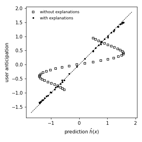
Quantifies the (subjective) explainability of a trained hypothesis for a simulated user, via the two measures discussed in the entry: the deviation between the user-anticipated and the actual predictions on a test set, and the empirical conditional entropy of the predictions given the user's anticipations. Providing explanations (LIME-style local linear approximations) raises both measures. Self-contained (numpy/matplotlib only), fixed seed.
Run it without installing anything:uv run https://dictionaryofml.org/terms/explainability.py
uv downloads this script and the pinned NumPy and Matplotlib it needs, then runs it; the script fetches any input file it uses. To keep the output files, download explainability.py into a folder and run uv run explainability.py there. With NumPy and Matplotlib already installed, python3 explainability.py, from any directory — it writes its output files into the current directory. Fixed seeds, so the printed numbers reproduce exactly. Download explainability.py · Notebook · Open in Colab
One cell per block of the script: the code, and what that code printed when it last ran here
"""
explainability.py — numerical companion to the glossary entry
'explainability'.

Purpose
-------
Quantifies the (subjective) explainability of a trained hypothesis for a
simulated user, via the two measures discussed in the entry: the deviation
between the user-anticipated and the actual predictions on a test set, and
the empirical conditional entropy of the predictions given the user's
anticipations.  Providing explanations (LIME-style local linear
approximations) raises both measures.  Self-contained (numpy/matplotlib
only), fixed seed.

Setup
-----
Trained hypothesis: Gaussian-kernel ridge regression fit to m = 30 noisy
samples of a nonlinear function on [-3, 3] — opaque to a user who reasons
in terms of linear maps.  The user is simulated as ridge-fitting a linear
map to a small set of labeled examples of the hypothesis' predictions
("mental model"), and anticipating predictions on a test set.

Blocks
------
[B-lin]    For a LINEAR trained hypothesis, the simulated user anticipates
           its test-set predictions almost exactly (mean squared deviation
           < 1e-3): a linear hypothesis is highly explainable to this user.
[B-opaque] For the kernel hypothesis, the user's anticipation deviates
           strongly (mean squared deviation > 0.1): low explainability.
[B-expl]   Explanations close the gap: given a LIME-style local linear
           approximation around each test point (fit to perturbations near
           the point), the user's anticipation error drops by a factor
           of at least 10 compared with [B-opaque].
[B-ent]    The empirical conditional entropy H(prediction | anticipation)
           (both discretized into 8 bins) is smaller with explanations
           than without: anticipations become more informative about the
           predictions.
[B-local]  One explanation shown in full: at the test point where the
           user's anticipation without explanations deviates most, the
           local linear approximation of the kernel hypothesis is written
           out, and the anticipation read from it lies within 0.1 of the
           prediction while the anticipation without explanations is off
           by more than 0.3.

Outputs
-------
explainability_scatter.csv : test-set points with columns yhat (prediction
                             of the kernel hypothesis), u_no (user
                             anticipation without explanations), u_expl
                             (with explanations), for the entry's pgfplots
                             figure.
explainability_local.csv   : grid x with columns h (kernel hypothesis),
                             u_glob (the user's linear mental model fitted
                             without explanations) and g_loc (the local
                             linear approximation at the point of [B-local]),
                             for the left panel of the entry's figure.
explainability_point.csv   : one row with that point x0, the prediction
                             yhat0 and the two anticipations u_no0, u_expl0.
explainability.png         : matplotlib preview of the two-panel figure
                             (checking only).
"""

import numpy as np
import matplotlib

matplotlib.use("Agg")
import matplotlib.pyplot as plt

from pathlib import Path

OUT_DIR = Path(__file__).parent

report = []


def check(name, ok):
    report.append((name, bool(ok)))
    print(f"  [{'ok' if ok else 'FAIL'}] {name}")


rng = np.random.default_rng(0)

# ------------------------------------------------- trained hypotheses
m = 30
x_tr = np.sort(rng.uniform(-3.0, 3.0, m))
y_tr = np.sin(1.5 * x_tr) + 0.5 * x_tr + 0.1 * rng.standard_normal(m)

SIGMA, ALPHA = 0.6, 1e-2


def gauss_kernel(p, q):
    return np.exp(-(p[:, None] - q[None, :]) ** 2 / (2.0 * SIGMA ** 2))


beta = np.linalg.solve(gauss_kernel(x_tr, x_tr) + ALPHA * m * np.eye(m),
                       y_tr)


def h_kernel(p):
    """Opaque hypothesis: Gaussian-kernel ridge regression."""
    return gauss_kernel(np.atleast_1d(p), x_tr) @ beta


w_lin = np.polyfit(x_tr, y_tr, 1)


def h_linear(p):
    """Interpretable hypothesis: linear map (with intercept)."""
    return np.polyval(w_lin, p)


def user_linear_fit(h, x_examples):
    """The simulated user ridge-fits a linear map (slope, intercept) to
    labeled examples of the hypothesis' predictions."""
    A = np.c_[x_examples, np.ones_like(x_examples)]
    return np.linalg.solve(A.T @ A + 1e-6 * np.eye(2), A.T @ h(x_examples))


def user_anticipation(h, x_examples, x_test):
    """The simulated user fits a linear map to labeled examples of the
    hypothesis' predictions and extrapolates to the test points."""
    w = user_linear_fit(h, x_examples)
    return np.c_[x_test, np.ones_like(x_test)] @ w


x_ex = np.linspace(-3.0, 3.0, 6)          # examples shown to the user
x_te = np.linspace(-2.8, 2.8, 40)         # test set to anticipate
For a LINEAR trained hypothesis, the simulated user anticipates its test-set predictions almost exactly (mean squared deviation < 1e-3): a linear hypothesis is highly explainable to this user.
dev_lin = float(np.mean(
    (user_anticipation(h_linear, x_ex, x_te) - h_linear(x_te)) ** 2))
check(f"[B-lin]    linear hypothesis anticipated (msd {dev_lin:.1e})",
      dev_lin < 1e-3)
[ok] [B-lin] linear hypothesis anticipated (msd 3.2e-15)
For the kernel hypothesis, the user's anticipation deviates strongly (mean squared deviation > 0.1): low explainability.
u_no = user_anticipation(h_kernel, x_ex, x_te)
yhat = h_kernel(x_te)
dev_no = float(np.mean((u_no - yhat) ** 2))
check(f"[B-opaque] kernel hypothesis not anticipated (msd {dev_no:.2f})",
      dev_no > 0.1)
[ok] [B-opaque] kernel hypothesis not anticipated (msd 0.51)
Explanations close the gap: given a LIME-style local linear approximation around each test point (fit to perturbations near the point), the user's anticipation error drops by a factor of at least 10 compared with [B-opaque].
u_expl = np.empty_like(x_te)
w_loc = np.empty((len(x_te), 2))             # local (slope, intercept)
for i, xt in enumerate(x_te):
    x_loc = xt + 0.25 * rng.standard_normal(20)   # LIME-style perturbations
    w_loc[i] = user_linear_fit(h_kernel, x_loc)
    u_expl[i] = w_loc[i] @ np.array([xt, 1.0])
dev_expl = float(np.mean((u_expl - yhat) ** 2))
check(f"[B-expl]   explanations shrink the deviation "
      f"({dev_no:.2f} -> {dev_expl:.4f})", dev_no > 10.0 * dev_expl)
[ok] [B-expl] explanations shrink the deviation (0.51 -> 0.0013)
The empirical conditional entropy H(prediction | anticipation) (both discretized into 8 bins) is smaller with explanations than without: anticipations become more informative about the predictions.
def cond_entropy(target, given, bins=8):
    """Empirical conditional entropy H(target | given) in bits."""
    lo, hi = min(target.min(), given.min()), max(target.max(), given.max())
    edges = np.linspace(lo, hi + 1e-9, bins + 1)
    t = np.digitize(target, edges) - 1
    g = np.digitize(given, edges) - 1
    joint = np.zeros((bins, bins))
    for ti, gi in zip(t, g):
        joint[ti, gi] += 1
    joint /= joint.sum()
    pg = joint.sum(axis=0)
    with np.errstate(divide="ignore", invalid="ignore"):
        cond = joint / pg[None, :]
        terms = np.where(joint > 0, joint * np.log2(cond), 0.0)
    return float(-terms.sum())


H_no = cond_entropy(yhat, u_no)
H_expl = cond_entropy(yhat, u_expl)
check(f"[B-ent]    conditional entropy drops ({H_no:.2f} -> {H_expl:.2f} "
      f"bits)", H_expl < H_no)
[ok] [B-ent] conditional entropy drops (1.22 -> 0.09 bits)
One explanation shown in full: at the test point where the user's anticipation without explanations deviates most, the local linear approximation of the kernel hypothesis is written out, and the anticipation read from it lies within 0.1 of the prediction while the anticipation without explanations is off by more than 0.3.
i0 = int(np.argmax(np.abs(u_no - yhat)))     # worst anticipation without
x0, yhat0, u_no0, u_expl0 = x_te[i0], yhat[i0], u_no[i0], u_expl[i0]
x_grid = np.linspace(-3.0, 3.0, 121)
w_glob = user_linear_fit(h_kernel, x_ex)     # the user's mental model
u_glob = np.c_[x_grid, np.ones_like(x_grid)] @ w_glob
g_loc = np.c_[x_grid, np.ones_like(x_grid)] @ w_loc[i0]
check(f"[B-local]  at x0={x0:.2f}: explanation {abs(u_expl0 - yhat0):.3f} "
      f"off, no explanation {abs(u_no0 - yhat0):.2f} off",
      abs(u_expl0 - yhat0) < 0.1 and abs(u_no0 - yhat0) > 0.3)

# ---------------------------------------------------------------- CSV
with open(OUT_DIR / "explainability_scatter.csv", "w") as f:
    f.write("yhat,u_no,u_expl\n")
    for a, b, c in zip(yhat, u_no, u_expl):
        f.write(f"{a:.4f},{b:.4f},{c:.4f}\n")
with open(OUT_DIR / "explainability_local.csv", "w") as f:
    f.write("x,h,u_glob,g_loc\n")
    for a, b, c, d in zip(x_grid, h_kernel(x_grid), u_glob, g_loc):
        f.write(f"{a:.4f},{b:.4f},{c:.4f},{d:.4f}\n")
with open(OUT_DIR / "explainability_point.csv", "w") as f:
    f.write("x0,yhat0,u_no0,u_expl0\n")
    f.write(f"{x0:.4f},{yhat0:.4f},{u_no0:.4f},{u_expl0:.4f}\n")

# -------------------------------------------------------------- preview
fig, (axl, ax) = plt.subplots(1, 2, figsize=(8.4, 4.2))
win = np.abs(x_grid - x0) <= 0.6
axl.plot(x_grid, h_kernel(x_grid), "k-", lw=1.2,
         label="prediction $\\hat{h}(x)$")
axl.plot(x_grid, u_glob, "k--", lw=0.8,
         label="user's linear mental model")
axl.plot(x_grid[win], g_loc[win], "-", color="0.55", lw=3,
         label="explanation: local linear approximation")
axl.axvline(x0, color="k", ls=":", lw=0.6)
axl.plot([x0], [u_no0], "ks", mfc="none", ms=6,
         label="anticipation without explanation")
axl.plot([x0], [u_expl0], "k.", ms=9, label="anticipation with explanation")
axl.set_xlabel("feature $x$")
axl.set_ylabel("label $y$")
axl.set_title(f"one explanation, at $x_0={x0:.2f}$")
axl.legend(frameon=False, fontsize=7, loc="lower right")
lim = [yhat.min() - 0.3, yhat.max() + 0.3]
ax.plot(lim, lim, "k--", lw=0.8)
ax.plot(yhat, u_no, "ks", mfc="none", ms=4, label="without explanations")
ax.plot(yhat, u_expl, "k.", ms=5, label="with explanations")
ax.set_xlabel("prediction $\\hat{h}(x)$")
ax.set_ylabel("user anticipation")
ax.set_title("explanations align user anticipation")
ax.legend(frameon=False, fontsize=8)
ax.set_aspect("equal")
fig.tight_layout()
fig.savefig(OUT_DIR / "explainability.png", dpi=110)

n_ok = sum(ok for _, ok in report)
print(f"\n{n_ok}/{len(report)} checks pass")
print(f"wrote {OUT_DIR / 'explainability_scatter.csv'}, "
      f"{OUT_DIR / 'explainability_local.csv'}, "
      f"{OUT_DIR / 'explainability_point.csv'}, "
      f"{OUT_DIR / 'explainability.png'}")
if n_ok != len(report):
    raise SystemExit(1)
  [ok] [B-local]  at x0=1.08: explanation 0.082 off, no explanation 1.19 off

5/5 checks pass
wrote /Users/junga1/dictionaryappliedml/pythondemos/explainability_scatter.csv, /Users/junga1/dictionaryappliedml/pythondemos/explainability_local.csv, /Users/junga1/dictionaryappliedml/pythondemos/explainability_point.csv, /Users/junga1/dictionaryappliedml/pythondemos/explainability.png
B-local writes when the script runs