B-plot writes when the script runsDictionary of Applied Machine Learning · deep net
Updated on 2026-11-20
Numerical companion to the entry deep net: it recomputes what the entry states and prints one line per check
Numerical companion to the glossary entry 'deepnet' (deep net). One feature per data point, the day of the year, and one label, the daily maximum temperature at Krems (GeoSphere station 3805). The maximum temperature rises until July and falls again towards December, so no linear hypothesis of the day index predicts it: least squares on that single feature stays just below the training error of the constant hypothesis that always predicts the sample mean of the training labels.
Run it without installing anything:uv run https://dictionaryofml.org/terms/deepnet.py
uv downloads this script and the pinned NumPy and Matplotlib it needs, then runs it; the script fetches any input file it uses. To keep the output files, download deepnet.py into a folder and run uv run deepnet.py there. With NumPy and Matplotlib already installed, python3 deepnet.py, from any directory — it writes its output files into the current directory. Fixed seeds, so the printed numbers reproduce exactly. Download deepnet.py · Notebook · Open in Colab
Before running a downloaded copy, scan it: uvx bandit -q -t B102,B307,B602,B605 deepnet.py (B102,B307,B602,B605 are the exec, eval and shell checks of bandit) reports nothing: the script runs no shell command and evaluates no generated code.
One cell per block of the script: the code, and what that code printed when it last ran here
"""A deep net as a composition of layers: the day of the year at Krems an
der Donau turned into learned features, and the training and validation
error of the net against its depth.

Purpose
-------
Numerical companion to the glossary entry 'deepnet' (deep net).  One
feature per data point, the day of the year, and one label, the daily
maximum temperature at Krems (GeoSphere station 3805).  The maximum
temperature rises until July and falls again towards December, so no
linear hypothesis of the day index predicts it: least squares on that
single feature stays just below the training error of the constant
hypothesis that always predicts the sample mean of the training labels.

A deep net of depth L is built here exactly as the entry defines it:
layer l applies the affine map W^(l) a^(l-1) + b^(l) to the activations
of the previous layer and then the rectified linear activation function
to every entry of the result, with a^(0) the raw feature vector, and the
last layer applies an affine map alone, so that the net output is a
linear hypothesis of the activations a^(L-1).  Nothing but numpy is
used: the forward pass is the composition, the gradient comes from
backpropagation (checked against a numerical gradient), and training
is plain gradient descent with a fixed learning rate and a fixed seed.

The nets are trained on the 365 days of 2023 and validated on the 366
days of 2024.  Depth 1 is the linear hypothesis; depth 2 already cuts
the training error by a factor of four; depth 3 to 5 keep lowering the
training error while the validation error rises again.  A separate net
of depth 3 whose last hidden layer has two neurons shows the
feature-learning reading: its two activations are two learned features
of the date, the net output is a linear hypothesis of them, and least
squares on those two features reaches almost the same training error as
the net's own output layer.

What the depth costs is measured too.  A feature transformation chosen
beforehand, the sine and cosine of the date at the annual period and at
half of it, needs five model parameters and reaches a lower validation
error than the depth-2 net with its 25.  And the training error of a net
is not a convex function of its model parameters, so gradient descent
returns a different hypothesis from every initialization: five
initializations of the same depth-2 net are trained here and their
training errors differ by more than a tenth.

Self-contained (numpy and matplotlib only), fixed seeds; the GeoSphere
download falls back to the committed CSV.

Blocks
------
[B-data]     Daily maximum temperature at Krems for 2023 and 2024 (731
             days, no missing value), and the single feature, the day of
             the year.
[B-net]      The net as a composition of layers: forward pass, the
             gradient by backpropagation checked against a numerical
             gradient, and gradient descent.
[B-depth]    Nets of depth 1 to 5 trained on the 2023 days; training
             error and validation error against the depth.
[B-curves]   The learned hypothesis maps of the depth-1, depth-2 and
             depth-5 nets over the year, and the 20 days of 2023 drawn
             in the entry's figure (every 18th day in calendar order).
[B-features] A depth-3 net whose last hidden layer has two neurons: the
             net output is a linear hypothesis of its two activations,
             and least squares on those two learned features reaches
             almost the same training error.
[B-limits]   What the depth costs: least squares on a feature
             transformation chosen beforehand, the sine and cosine of
             the date, against the depth-2 net; and the spread of the
             training error over five initializations of one net.
[B-plot]     Preview: the hypothesis maps over the year, and the two
             errors against the depth.

Outputs
-------
deepnet_weather.csv   : date, day of the year, maximum temperature for
                        2023 and 2024 (committed copy of the download).
deepnet_depth.csv     : depth, training error, validation error.
deepnet_curves.csv    : day of the year, prediction of the depth-1,
                        depth-2 and depth-5 net, in degrees Celsius.
deepnet_days_plot.csv : the 20 days of 2023 drawn in the entry's figure.
deepnet.png           : matplotlib preview (checking only).
"""

# /// script
# requires-python = ">=3.10"
# dependencies = ["matplotlib==3.10.7", "numpy==2.3.4"]
# ///

import datetime
import json
import urllib.request
from pathlib import Path

import numpy as np
import matplotlib

matplotlib.use("Agg")
import matplotlib.pyplot as plt

OUT_DIR = Path(__file__).parent

report = []                         # collects (check name, pass/fail) pairs


def check(name, ok):                # records and prints one verification
    report.append((name, bool(ok)))
    print(f"  [{'ok' if ok else 'FAIL'}] {name}")
Installed 11 packages in 59ms
Daily maximum temperature at Krems for 2023 and 2024 (731 days, no missing value), and the single feature, the day of the year.
print("[B-data] daily maximum temperature at Krems, 2023 and 2024")
URL = ("https://dataset.api.hub.geosphere.at/v1/station/historical/"
       "klima-v2-1d?parameters=tlmax&station_ids=3805"
       "&start=2023-01-01&end=2024-12-31")
CSV = OUT_DIR / "deepnet_weather.csv"


def day_of_year(stamp):
    return datetime.date(*map(int, stamp.split("-"))).timetuple().tm_yday


try:
    with urllib.request.urlopen(URL, timeout=120) as resp:
        payload = json.load(resp)
    series = payload["features"][0]["properties"]["parameters"]["tlmax"]
    records = [(stamp[:10], day_of_year(stamp[:10]), hi)
               for stamp, hi in zip(payload["timestamps"], series["data"])]
    with open(CSV, "w") as fh:
        fh.write("date,doy,tmax\n")
        for day, doy, hi in records:
            fh.write(f"{day},{doy},{hi}\n")
    print(f"    downloaded {len(records)} days")
except OSError as err:
    print(f"    download failed ({err}); reading the committed CSV")
    rows = CSV.read_text().strip().splitlines()[1:]
    records = [(d, int(n), float(v))
               for d, n, v in (r.split(",") for r in rows)]

check("[B-data] 731 days for 2023 and 2024", len(records) == 731)
check("[B-data] every day carries a maximum temperature",
      all(hi is not None for _, _, hi in records))
check("[B-data] the record matches the archive (1 July 2023: 24.9 deg, "
      "day 182 of the year)",
      records[181][:2] == ("2023-07-01", 182)
      and abs(records[181][2] - 24.9) < 1e-9)

dates = [d for d, _, _ in records]
doy = np.array([n for _, n, _ in records], dtype=float)
tmax = np.array([v for _, _, v in records], dtype=float)
is23 = np.array([d.startswith("2023") for d in dates])
# the single feature of a day, the day of the year, centered on 2 July and
# scaled so that the training feature values fill about [-1.7, 1.7]
FEAT_OFFSET, FEAT_SCALE = 183.0, 105.0
X = ((doy - FEAT_OFFSET) / FEAT_SCALE)[:, None]
# the label is centered on the training sample mean, which leaves every
# squared error unchanged and lets one learning rate serve every depth
LABEL_MEAN = float(tmax[is23].mean())
y = tmax - LABEL_MEAN
X_train, y_train = X[is23], y[is23]
X_val, y_val = X[~is23], y[~is23]
err_const = float((y_val ** 2).mean())
print(f"    sample mean of the 2023 labels {LABEL_MEAN:.2f} degrees; the "
      f"constant hypothesis has validation error {err_const:.1f}")
check("[B-data] 365 training days in 2023 and 366 validation days in 2024",
      len(y_train) == 365 and len(y_val) == 366)
[B-data] daily maximum temperature at Krems, 2023 and 2024
    downloaded 731 days
  [ok] [B-data] 731 days for 2023 and 2024
  [ok] [B-data] every day carries a maximum temperature
  [ok] [B-data] the record matches the archive (1 July 2023: 24.9 deg, day 182 of the year)
    sample mean of the 2023 labels 17.44 degrees; the constant hypothesis has validation error 84.9
  [ok] [B-data] 365 training days in 2023 and 366 validation days in 2024
The net as a composition of layers: forward pass, the gradient by backpropagation checked against a numerical gradient, and gradient descent.
print("[B-net] the net as a composition of layers; gradient by "
      "backpropagation")


def init(widths, seed):
    """Weight matrices and offset vectors of a net with the given widths."""
    rng = np.random.default_rng(seed)
    mats = [rng.standard_normal((nxt, prv)) * np.sqrt(2.0 / prv)
            for prv, nxt in zip(widths[:-1], widths[1:])]
    offs = [rng.standard_normal(nxt) * 0.5 for nxt in widths[1:]]
    return mats, offs


def forward(mats, offs, feats):
    """Activations of every layer: an affine map followed by the rectified
    linear activation function, applied to every entry, and an affine map
    alone in the last layer."""
    acts = [feats.T]
    depth = len(mats)
    for ell in range(depth):
        pre = mats[ell] @ acts[-1] + offs[ell][:, None]
        acts.append(np.maximum(pre, 0.0) if ell < depth - 1 else pre)
    return acts


def predict(mats, offs, feats):
    return forward(mats, offs, feats)[-1][0]


def average_loss(mats, offs, feats, labels):
    """Average squared error loss of the net on the given data points."""
    return float(((predict(mats, offs, feats) - labels) ** 2).mean())


def backprop(mats, offs, feats, labels):
    """The gradient of the average squared error loss with respect to
    every weight matrix and offset vector, one layer at a time."""
    acts = forward(mats, offs, feats)
    depth = len(mats)
    g = (2.0 / len(labels)) * (acts[-1][0] - labels)[None, :]
    d_mats, d_offs = [None] * depth, [None] * depth
    for ell in range(depth - 1, -1, -1):
        d_mats[ell] = g @ acts[ell].T
        d_offs[ell] = g.sum(axis=1)
        if ell > 0:
            g = (mats[ell].T @ g) * (acts[ell] > 0)
    return d_mats, d_offs


LRATE, NRITER = 0.01, 20000


def train(widths, seed=1):
    """Gradient descent on the training error, from the fixed-seed start."""
    mats, offs = init(widths, seed)
    for _ in range(NRITER):
        d_mats, d_offs = backprop(mats, offs, X_train, y_train)
        for ell in range(len(mats)):
            mats[ell] -= LRATE * d_mats[ell]
            offs[ell] -= LRATE * d_offs[ell]
    return mats, offs


mats0, offs0 = init([1, 8, 2, 1], 1)
d_mats0, _ = backprop(mats0, offs0, X_train, y_train)
EPS = 1e-6
rel = 0.0
rng_check = np.random.default_rng(7)
for ell in range(len(mats0)):
    for _ in range(5):
        i = int(rng_check.integers(mats0[ell].shape[0]))
        j = int(rng_check.integers(mats0[ell].shape[1]))
        mats0[ell][i, j] += EPS
        up = average_loss(mats0, offs0, X_train, y_train)
        mats0[ell][i, j] -= 2 * EPS
        down = average_loss(mats0, offs0, X_train, y_train)
        mats0[ell][i, j] += EPS
        numeric = (up - down) / (2 * EPS)
        rel = max(rel, abs(numeric - d_mats0[ell][i, j]) / max(1.0, abs(numeric)))
print(f"    largest relative deviation over 15 weights: {rel:.2e}")
check("[B-net] backpropagation agrees with the numerical gradient",
      rel < 1e-6)
one = np.array([[0.4]])
acts_one = forward(*init([1, 8, 2, 1], 1), one)
check("[B-net] every hidden activation is nonnegative, the last layer is "
      "affine only",
      all((a >= 0).all() for a in acts_one[1:-1]) and acts_one[-1].shape == (1, 1))
[B-net] the net as a composition of layers; gradient by backpropagation
    largest relative deviation over 15 weights: 4.99e-09
  [ok] [B-net] backpropagation agrees with the numerical gradient
  [ok] [B-net] every hidden activation is nonnegative, the last layer is affine only
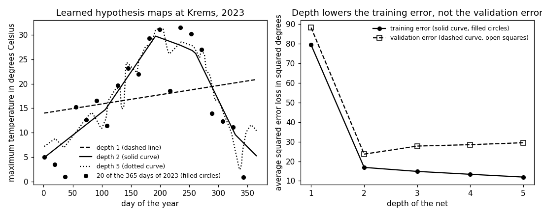
Nets of depth 1 to 5 trained on the 2023 days; training error and validation error against the depth.
print("[B-depth] nets of depth 1 to 5 trained on the 2023 days")
WIDTH, DEPTHS = 8, [1, 2, 3, 4, 5]
nets, err_train, err_val = {}, {}, {}
for depth in DEPTHS:
    widths = [1] + [WIDTH] * (depth - 1) + [1]
    nets[depth] = train(widths)
    err_train[depth] = average_loss(*nets[depth], X_train, y_train)
    err_val[depth] = average_loss(*nets[depth], X_val, y_val)
    print(f"    depth {depth} (widths {widths}): training error "
          f"{err_train[depth]:.1f}, validation error {err_val[depth]:.1f}")
with open(OUT_DIR / "deepnet_depth.csv", "w") as fh:
    fh.write("depth,trainerr,valerr\n")
    for depth in DEPTHS:
        fh.write(f"{depth},{err_train[depth]:.2f},{err_val[depth]:.2f}\n")
check("[B-depth] the depth-1 net is a linear hypothesis and stays within "
      "6 percent of the constant hypothesis on the training days",
      abs(err_train[1] - float((y_train ** 2).mean())) / err_train[1] < 0.06)
check("[B-depth] one hidden layer cuts the training error by at least a "
      "factor of four", err_train[1] > 4 * err_train[2])
check("[B-depth] the training error falls with every added layer",
      all(err_train[a] > err_train[b] for a, b in zip(DEPTHS, DEPTHS[1:])))
check("[B-depth] the validation error is smallest at depth 2 and rises "
      "with every further layer",
      min(err_val, key=err_val.get) == 2
      and all(err_val[a] < err_val[b] for a, b in zip(DEPTHS[1:], DEPTHS[2:])))
[B-depth] nets of depth 1 to 5 trained on the 2023 days
    depth 1 (widths [1, 1]): training error 79.4, validation error 88.2
    depth 2 (widths [1, 8, 1]): training error 16.9, validation error 23.7
    depth 3 (widths [1, 8, 8, 1]): training error 14.8, validation error 27.8
    depth 4 (widths [1, 8, 8, 8, 1]): training error 13.4, validation error 28.5
    depth 5 (widths [1, 8, 8, 8, 8, 1]): training error 12.0, validation error 29.5
  [ok] [B-depth] the depth-1 net is a linear hypothesis and stays within 6 percent of the constant hypothesis on the training days
  [ok] [B-depth] one hidden layer cuts the training error by at least a factor of four
  [ok] [B-depth] the training error falls with every added layer
  [ok] [B-depth] the validation error is smallest at depth 2 and rises with every further layer
The learned hypothesis maps of the depth-1, depth-2 and depth-5 nets over the year, and the 20 days of 2023 drawn in the entry's figure (every 18th day in calendar order).
print("[B-curves] the learned hypothesis maps over the year")
grid_doy = np.arange(1, 366, dtype=float)
grid_X = ((grid_doy - FEAT_OFFSET) / FEAT_SCALE)[:, None]
curves = {d: predict(*nets[d], grid_X) + LABEL_MEAN for d in (1, 2, 5)}
with open(OUT_DIR / "deepnet_curves.csv", "w") as fh:
    fh.write("doy,h1,h2,h5\n")
    for k, n in enumerate(grid_doy):
        fh.write(f"{int(n)},{curves[1][k]:.3f},{curves[2][k]:.3f},"
                 f"{curves[5][k]:.3f}\n")
check("[B-curves] the depth-1 hypothesis is a straight line in the day "
      "index (second differences vanish)",
      np.allclose(np.diff(curves[1], 2), 0.0, atol=1e-9))
peak2 = int(grid_doy[int(np.argmax(curves[2]))])
print(f"    the depth-2 hypothesis peaks on day {peak2} at "
      f"{curves[2].max():.1f} degrees, and ranges over "
      f"{curves[2].max() - curves[2].min():.1f} degrees; the depth-1 "
      f"hypothesis ranges over {curves[1].max() - curves[1].min():.1f}")
check("[B-curves] the depth-2 hypothesis peaks in July or August",
      182 <= peak2 <= 243)
# the entry's figure draws 20 of the 365 training days, every 18th day
# in calendar order, so that the single points stay legible
drawn = np.flatnonzero(is23)[::18][:20]
with open(OUT_DIR / "deepnet_days_plot.csv", "w") as fh:
    fh.write("doy,tmax\n")
    for k in drawn:
        fh.write(f"{int(doy[k])},{tmax[k]:.1f}\n")
check("[B-curves] 20 days drawn, every 18th day of 2023 from 1 January",
      len(drawn) == 20 and doy[drawn[0]] == 1 and doy[drawn[1]] == 19)
[B-curves] the learned hypothesis maps over the year
  [ok] [B-curves] the depth-1 hypothesis is a straight line in the day index (second differences vanish)
    the depth-2 hypothesis peaks on day 192 at 29.8 degrees, and ranges over 24.9 degrees; the depth-1 hypothesis ranges over 6.9
  [ok] [B-curves] the depth-2 hypothesis peaks in July or August
  [ok] [B-curves] 20 days drawn, every 18th day of 2023 from 1 January
A depth-3 net whose last hidden layer has two neurons: the net output is a linear hypothesis of its two activations, and least squares on those two learned features reaches almost the same training error.
print("[B-features] a depth-3 net whose last hidden layer has two neurons")
mats_f, offs_f = train([1, WIDTH, 2, 1], seed=2)
Z_train = forward(mats_f, offs_f, X_train)[-2].T        # 365 x 2
Z_val = forward(mats_f, offs_f, X_val)[-2].T
out_train = predict(mats_f, offs_f, X_train)
linear_on_Z = Z_train @ mats_f[-1][0] + offs_f[-1][0]
check("[B-features] the net output is the linear hypothesis of the two "
      "activations given by the last layer",
      np.allclose(out_train, linear_on_Z))
check("[B-features] both learned features vary over the training days",
      (Z_train.std(axis=0) > 1e-6).all())
A_train = np.hstack([Z_train, np.ones((len(Z_train), 1))])
w_ls = np.linalg.lstsq(A_train, y_train, rcond=None)[0]
err_net = average_loss(mats_f, offs_f, X_train, y_train)
err_ls = float(((A_train @ w_ls - y_train) ** 2).mean())
A_val = np.hstack([Z_val, np.ones((len(Z_val), 1))])
err_ls_val = float(((A_val @ w_ls - y_val) ** 2).mean())
raw = np.hstack([X_train, np.ones((len(X_train), 1))])
w_raw = np.linalg.lstsq(raw, y_train, rcond=None)[0]
err_raw = float(((raw @ w_raw - y_train) ** 2).mean())
print(f"    training error of the net {err_net:.2f}, of least squares on "
      f"its two learned features {err_ls:.2f}, of least squares on the raw "
      f"feature {err_raw:.2f}")
print(f"    validation error of the net "
      f"{average_loss(mats_f, offs_f, X_val, y_val):.2f}, of least squares "
      f"on the two learned features {err_ls_val:.2f}")
check("[B-features] least squares on the two learned features cannot beat "
      "the net's own output layer by more than 1 percent",
      err_ls <= err_net and err_net - err_ls < 0.01 * err_net)
check("[B-features] the two learned features carry most of what the raw "
      "feature does not: least squares on them has less than a third of "
      "the training error", err_ls < err_raw / 3)
[B-features] a depth-3 net whose last hidden layer has two neurons
  [ok] [B-features] the net output is the linear hypothesis of the two activations given by the last layer
  [ok] [B-features] both learned features vary over the training days
    training error of the net 14.61, of least squares on its two learned features 14.54, of least squares on the raw feature 79.43
    validation error of the net 26.03, of least squares on the two learned features 25.91
  [ok] [B-features] least squares on the two learned features cannot beat the net's own output layer by more than 1 percent
  [ok] [B-features] the two learned features carry most of what the raw feature does not: least squares on them has less than a third of the training error
What the depth costs: least squares on a feature transformation chosen beforehand, the sine and cosine of the date, against the depth-2 net; and the spread of the training error over five initializations of one net.
# ---- spread over initializations
print("[B-limits] least squares on the sine and cosine of the date, and "
      "five initializations of the depth-2 net")
PERIOD = 2.0 * np.pi / 365.0


def chosen_features(days):
    """The feature transformation chosen beforehand: the sine and cosine of
    the date at the annual period and at half of it, and a constant."""
    return np.column_stack([np.sin(PERIOD * days), np.cos(PERIOD * days),
                            np.sin(2 * PERIOD * days),
                            np.cos(2 * PERIOD * days),
                            np.ones(len(days))])


C_train, C_val = chosen_features(doy[is23]), chosen_features(doy[~is23])
w_chosen = np.linalg.lstsq(C_train, y_train, rcond=None)[0]
err_chosen_train = float(((C_train @ w_chosen - y_train) ** 2).mean())
err_chosen_val = float(((C_val @ w_chosen - y_val) ** 2).mean())
nr_param_net2 = sum(m.size for m in nets[2][0]) + sum(
    o.size for o in nets[2][1])
print(f"    chosen transformation ({w_chosen.size} model parameters): "
      f"training error {err_chosen_train:.1f}, validation error "
      f"{err_chosen_val:.1f}")
print(f"    depth-2 net ({nr_param_net2} model parameters): training error "
      f"{err_train[2]:.1f}, validation error {err_val[2]:.1f}")
check("[B-limits] the chosen transformation has a lower validation error "
      "than the depth-2 net, with fewer model parameters",
      err_chosen_val < err_val[2] and w_chosen.size < nr_param_net2)
check("[B-limits] the depth-2 net still has the lower training error, so "
      "the chosen transformation is not simply the larger model",
      err_train[2] < err_chosen_train)
raw_val = np.hstack([X_val, np.ones((len(X_val), 1))])
err_raw_val = float(((raw_val @ w_raw - y_val) ** 2).mean())
print(f"    least squares on the raw feature (2 model parameters): "
      f"training error {err_raw:.1f}, validation error {err_raw_val:.1f}")
check("[B-limits] least squares on the raw feature has the validation "
      "error of the depth-1 net, which is the same linear hypothesis",
      abs(err_raw_val - err_val[1]) < 0.05)

SEEDS = [1, 2, 3, 4, 5]
seed_train, seed_val = [], []
for seed in SEEDS:
    mats_s, offs_s = train([1, WIDTH, 1], seed=seed)
    seed_train.append(average_loss(mats_s, offs_s, X_train, y_train))
    seed_val.append(average_loss(mats_s, offs_s, X_val, y_val))
print("    five initializations of the depth-2 net, training error: "
      + ", ".join(f"{v:.1f}" for v in seed_train))
print("    the same five, validation error: "
      + ", ".join(f"{v:.1f}" for v in seed_val))
check("[B-limits] the five initializations give five different training "
      "errors", len({round(v, 6) for v in seed_train}) == 5)
check("[B-limits] the largest of the five training errors exceeds the "
      "smallest by more than a tenth",
      max(seed_train) > 1.1 * min(seed_train))
check("[B-limits] four of the five end above the smallest training error "
      "the five reach, so a single run cannot be relied on to return the "
      "best hypothesis of the net",
      sum(v > min(seed_train) for v in seed_train) == 4)
check("[B-limits] the first of the five repeats the depth-2 net of the "
      "depth block, which starts from the same initialization",
      abs(seed_train[0] - err_train[2]) < 1e-9)
[B-limits] least squares on the sine and cosine of the date, and five initializations of the depth-2 net
    chosen transformation (5 model parameters): training error 17.3, validation error 22.6
    depth-2 net (25 model parameters): training error 16.9, validation error 23.7
  [ok] [B-limits] the chosen transformation has a lower validation error than the depth-2 net, with fewer model parameters
  [ok] [B-limits] the depth-2 net still has the lower training error, so the chosen transformation is not simply the larger model
    least squares on the raw feature (2 model parameters): training error 79.4, validation error 88.2
  [ok] [B-limits] least squares on the raw feature has the validation error of the depth-1 net, which is the same linear hypothesis
    five initializations of the depth-2 net, training error: 16.9, 19.1, 16.9, 19.1, 18.1
    the same five, validation error: 23.7, 23.1, 23.6, 23.2, 24.7
  [ok] [B-limits] the five initializations give five different training errors
  [ok] [B-limits] the largest of the five training errors exceeds the smallest by more than a tenth
  [ok] [B-limits] four of the five end above the smallest training error the five reach, so a single run cannot be relied on to return the best hypothesis of the net
  [ok] [B-limits] the first of the five repeats the depth-2 net of the depth block, which starts from the same initialization
Preview: the hypothesis maps over the year, and the two errors against the depth.
print("[B-plot] preview")
fig, (ax1, ax2) = plt.subplots(1, 2, figsize=(10, 4))
ax1.plot(grid_doy, curves[1], "k--", label="depth 1 (dashed line)")
ax1.plot(grid_doy, curves[2], "k-", label="depth 2 (solid curve)")
ax1.plot(grid_doy, curves[5], "k:", label="depth 5 (dotted curve)")
ax1.plot(doy[drawn], tmax[drawn], "ko", ms=5,
         label="20 of the 365 days of 2023 (filled circles)")
ax1.set_xlabel("day of the year")
ax1.set_ylabel("maximum temperature in degrees Celsius")
ax1.set_title("Learned hypothesis maps at Krems, 2023")
ax1.legend(frameon=False, fontsize=8)
ax2.plot(DEPTHS, [err_train[d] for d in DEPTHS], "k-o", ms=5,
         label="training error (solid curve, filled circles)")
ax2.plot(DEPTHS, [err_val[d] for d in DEPTHS], "k--s", ms=6,
         markerfacecolor="none", label="validation error (dashed curve, "
         "open squares)")
ax2.set_xlabel("depth of the net")
ax2.set_ylabel("average squared error loss in squared degrees")
ax2.set_title("Depth lowers the training error, not the validation error")
ax2.set_xticks(DEPTHS)
ax2.legend(frameon=False, fontsize=8)
fig.tight_layout()
fig.savefig(OUT_DIR / "deepnet.png", dpi=110)

print()
failed = [n for n, ok in report if not ok]
print(f"{len(report) - len(failed)}/{len(report)} checks passed"
      + (f"; FAILED: {failed}" if failed else ""))
[B-plot] preview

24/24 checks passed
B-plot writes when the script runs