B-clean writes when the script runsDictionary of Applied Machine Learning · data leakage
Numerical companion to the entry data leakage: it recomputes what the entry states and prints one line per check
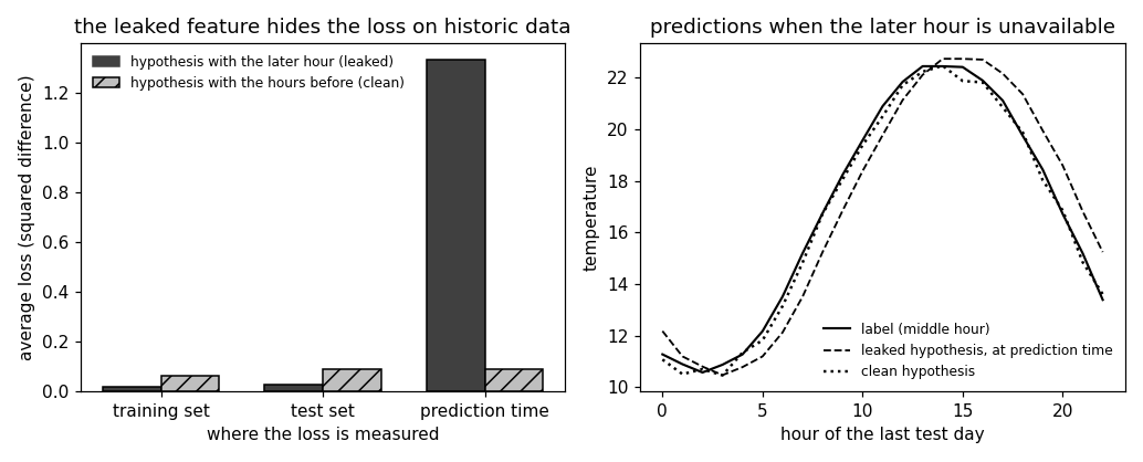
Reproduces the entry's example: an hourly temperature sequence, each data point a sliding window of three consecutive hours, the label the temperature of the middle hour. A hypothesis that uses the measurement one hour LATER as a feature has a loss near zero on the training set and the test set, because on historic data that measurement is available; at prediction time it is not, and the same hypothesis fails. A hypothesis that uses only the two hours BEFORE the middle hour has the same loss on historic data and at prediction time. Self-contained (numpy/matplotlib only), fixed seed.
Run it without installing anything:uv run https://dictionaryofml.org/terms/dataleakage.py
uv downloads this script and the pinned NumPy and Matplotlib it needs, then runs it; the script fetches any input file it uses. To keep the output files, download dataleakage.py into a folder and run uv run dataleakage.py there. With NumPy and Matplotlib already installed, python3 dataleakage.py, from any directory — it writes its output files into the current directory. Fixed seeds, so the printed numbers reproduce exactly. Download dataleakage.py · Notebook · Open in Colab
One cell per block of the script: the code, and what that code printed when it last ran here
"""
dataleakage.py — numerical companion to the glossary entry 'data leakage'.

Purpose
-------
Reproduces the entry's example: an hourly temperature sequence, each
data point a sliding window of three consecutive hours, the label the
temperature of the middle hour.  A hypothesis that uses the measurement
one hour LATER as a feature has a loss near zero on the training set and
the test set, because on historic data that measurement is available;
at prediction time it is not, and the same hypothesis fails.  A
hypothesis that uses only the two hours BEFORE the middle hour has the
same loss on historic data and at prediction time.  Self-contained
(numpy/matplotlib only), fixed seed.

Setup
-----
Sequence: 480 hourly temperatures (20 days) with a daily cycle, a slow
trend and measurement noise (variance 0.01).  Each window gives the label y = temperature
of the middle hour and two candidate feature sets:
  leaked : (one hour before, one hour LATER)   -- the later hour leaks
  clean  : (two hours before, one hour before) -- available in real time
The hypothesis is a weighted sum of the features plus an offset, fitted
by minimizing the average loss on the first 14 days (training set); the
loss is the squared difference between label and prediction.  The last
6 days are the test set.  At prediction time the later hour has not been
measured, so its slot can only hold the latest available measurement,
the hour before the middle hour.

Blocks
------
[B-leak]   On historic data the leaked hypothesis looks excellent: its
           average loss on the training set and on the test set is below
           0.03, close to the noise level 0.01.
[B-deploy] At prediction time the later hour is unavailable; filling its
           slot with the latest measurement raises the test loss of the
           leaked hypothesis by a factor above 10, far above the clean
           hypothesis.
[B-clean]  The clean hypothesis has the same loss on the test set and at
           prediction time (identical by construction), and that loss is
           below the deployed loss of the leaked hypothesis.

Outputs
-------
dataleakage_losses.csv : one row per hypothesis (leaked, clean) with the
                         average loss on the training set, on the test
                         set, and at prediction time.
dataleakage_window.csv : the last test day, hour by hour: label and the
                         predictions of both hypotheses at prediction
                         time (for a figure of the sequence).
dataleakage.png        : matplotlib preview (checking only).
"""

import numpy as np
import matplotlib

matplotlib.use("Agg")
import matplotlib.pyplot as plt

from pathlib import Path

OUT_DIR = Path(__file__).parent

report = []


def check(name, ok):
    report.append((name, bool(ok)))
    print(f"  [{'ok' if ok else 'FAIL'}] {name}")


rng = np.random.default_rng(0)

# ---------------------------------------------------------------- sequence
n_hours = 480                                   # 20 days
t = np.arange(n_hours)
temp = (12.0 + 6.0 * np.sin(2 * np.pi * (t - 8) / 24) + 0.01 * t
        + 0.1 * rng.standard_normal(n_hours))   # noise variance 0.01

# windows: middle hour i, label temp[i]; "later" = temp[i+1]
i = np.arange(2, n_hours - 1)
y = temp[i]
X_leak = np.c_[temp[i - 1], temp[i + 1], np.ones_like(y)]      # before, LATER
X_clean = np.c_[temp[i - 2], temp[i - 1], np.ones_like(y)]     # two before
train = i < 14 * 24
test = ~train


def fit(X, y):
    return np.linalg.lstsq(X, y, rcond=None)[0]


def loss(w, X, y):
    return float(np.mean((y - X @ w) ** 2))


w_leak = fit(X_leak[train], y[train])
w_clean = fit(X_clean[train], y[train])
On historic data the leaked hypothesis looks excellent: its average loss on the training set and on the test set is below 0.03, close to the noise level 0.01.
l_leak_tr, l_leak_te = loss(w_leak, X_leak[train], y[train]), loss(w_leak, X_leak[test], y[test])
check(f"[B-leak]   leaked hypothesis on historic data: training loss "
      f"{l_leak_tr:.3f}, test loss {l_leak_te:.3f} (noise level 0.01)",
      l_leak_tr < 0.03 and l_leak_te < 0.03)
[ok] [B-leak] leaked hypothesis on historic data: training loss 0.017, test loss 0.025 (noise level 0.01)
At prediction time the later hour is unavailable; filling its slot with the latest measurement raises the test loss of the leaked hypothesis by a factor above 10, far above the clean hypothesis.
# at prediction time the later hour is unknown: its slot holds the latest
# measurement, the hour before the middle hour
X_leak_deploy = np.c_[temp[i - 1], temp[i - 1], np.ones_like(y)]
l_leak_dep = loss(w_leak, X_leak_deploy[test], y[test])
l_clean_te = loss(w_clean, X_clean[test], y[test])
check(f"[B-deploy] at prediction time the leaked hypothesis has test loss "
      f"{l_leak_dep:.2f}, {l_leak_dep / l_leak_te:.0f} times its historic "
      f"test loss", l_leak_dep > 10 * l_leak_te and l_leak_dep > l_clean_te)
[ok] [B-deploy] at prediction time the leaked hypothesis has test loss 1.33, 53 times its historic test loss
The clean hypothesis has the same loss on the test set and at prediction time (identical by construction), and that loss is below the deployed loss of the leaked hypothesis.
l_clean_tr = loss(w_clean, X_clean[train], y[train])
l_clean_dep = loss(w_clean, X_clean[test], y[test])     # same features
check(f"[B-clean]  clean hypothesis: training loss {l_clean_tr:.2f}, test "
      f"loss {l_clean_te:.2f}, at prediction time {l_clean_dep:.2f} "
      f"(unchanged); leaked hypothesis at prediction time {l_leak_dep:.2f}",
      abs(l_clean_te - l_clean_dep) < 1e-12 and l_clean_dep < l_leak_dep)

# ---------------------------------------------------------------- CSV
with open(OUT_DIR / "dataleakage_losses.csv", "w") as fh:
    fh.write("hypothesis,train,test,deployed\n")
    fh.write(f"leaked,{l_leak_tr:.4f},{l_leak_te:.4f},{l_leak_dep:.4f}\n")
    fh.write(f"clean,{l_clean_tr:.4f},{l_clean_te:.4f},{l_clean_dep:.4f}\n")
last = (i >= n_hours - 24) & (i < n_hours - 1)
with open(OUT_DIR / "dataleakage_window.csv", "w") as fh:
    fh.write("hour,label,pred_leaked_deployed,pred_clean\n")
    for h, a, b, c in zip(i[last] - (n_hours - 24), y[last],
                          X_leak_deploy[last] @ w_leak, X_clean[last] @ w_clean):
        fh.write(f"{h},{a:.3f},{b:.3f},{c:.3f}\n")

# -------------------------------------------------------------- preview
fig, (ax, ax2) = plt.subplots(1, 2, figsize=(9.4, 3.8))
from matplotlib.patches import Patch
pos = np.arange(3)
xs = np.r_[pos - 0.18, pos + 0.18]            # six bars, offset in pairs
vals = [l_leak_tr, l_leak_te, l_leak_dep, l_clean_tr, l_clean_te, l_clean_dep]
bars = ax.bar(xs, vals, 0.36, color=["0.25"] * 3 + ["0.75"] * 3, edgecolor="k")
for b in bars[3:]:
    b.set_hatch("//")
ax.set_xticks(pos); ax.set_xticklabels(["training set", "test set", "prediction time"])
ax.legend(handles=[Patch(color="0.25", label="hypothesis with the later hour (leaked)"),
                   Patch(facecolor="0.75", edgecolor="k", hatch="//",
                         label="hypothesis with the hours before (clean)")],
          frameon=False, fontsize=8)
ax.set_ylabel("average loss (squared difference)")
ax.set_xlabel("where the loss is measured")
ax.set_title("the leaked feature hides the loss on historic data")
hh = i[last] - (n_hours - 24)
ax2.plot(hh, y[last], "k-", lw=1.4, label="label (middle hour)")
ax2.plot(hh, X_leak_deploy[last] @ w_leak, "k--", lw=1.2, label="leaked hypothesis, at prediction time")
ax2.plot(hh, X_clean[last] @ w_clean, "k:", lw=1.6, label="clean hypothesis")
ax2.set_xlabel("hour of the last test day")
ax2.set_ylabel("temperature")
ax2.set_title("predictions when the later hour is unavailable")
ax2.legend(frameon=False, fontsize=8)
fig.tight_layout()
fig.savefig(OUT_DIR / "dataleakage.png", dpi=110)

n_ok = sum(ok for _, ok in report)
print(f"\n{n_ok}/{len(report)} checks pass")
print(f"wrote {OUT_DIR / 'dataleakage_losses.csv'}, {OUT_DIR / 'dataleakage_window.csv'}, "
      f"{OUT_DIR / 'dataleakage.png'}")
if n_ok != len(report):
    raise SystemExit(1)
  [ok] [B-clean]  clean hypothesis: training loss 0.06, test loss 0.09, at prediction time 0.09 (unchanged); leaked hypothesis at prediction time 1.33

3/3 checks pass
wrote /Users/junga1/dictionaryappliedml/pythondemos/dataleakage_losses.csv, /Users/junga1/dictionaryappliedml/pythondemos/dataleakage_window.csv, /Users/junga1/dictionaryappliedml/pythondemos/dataleakage.png
B-clean writes when the script runs