B-edge writes when the script runsDictionary of Applied Machine Learning · data imputation
Numerical companion to the entry data imputation: it recomputes what the entry states and prints one line per check
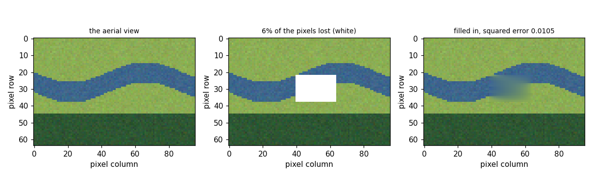
The entry's construction, carried out: an aerial photograph loses a rectangular region, and the lost pixels are filled in by learning to predict the RGB values of a pixel from the RGB values of its neighbors. Every intact pixel is one data point, its feature vector holds the RGB values of the eight surrounding pixels, and its label is its own RGB triple. Self-contained (numpy/matplotlib only), fixed seed.
Run it without installing anything:uv run https://dictionaryofml.org/terms/dataimputation.py
uv downloads this script and the pinned NumPy and Matplotlib it needs, then runs it; the script fetches any input file it uses. To keep the output files, download dataimputation.py into a folder and run uv run dataimputation.py there. With NumPy and Matplotlib already installed, python3 dataimputation.py, from any directory — it writes its output files into the current directory. Fixed seeds, so the printed numbers reproduce exactly. Download dataimputation.py · Notebook · Open in Colab
One cell per block of the script: the code, and what that code printed when it last ran here
"""
dataimputation.py -- numerical companion to the glossary entry
'data imputation'.

The entry's construction, carried out: an aerial photograph loses a
rectangular region, and the lost pixels are filled in by learning to
predict the RGB values of a pixel from the RGB values of its neighbors.
Every intact pixel is one data point, its feature vector holds the RGB
values of the eight surrounding pixels, and its label is its own RGB
triple. Self-contained (numpy/matplotlib only), fixed seed.

The photograph is synthetic. It stands in for an aerial view of the
Rossatz area on the Danube and is built to carry what matters here: wide
regions of nearly constant color (river, meadow, forest) separated by
sharp boundaries, so that a neighbor is informative inside a region and
misleading across a boundary.

Blocks
------
[B-scene]  The synthetic aerial view and the rectangular region whose
           pixels are lost, with the share of pixels that went missing.
[B-set]    Imputation read as a prediction task: every intact pixel
           whose eight neighbors are also intact becomes a data point,
           with a feature vector of 24 numbers and a label of 3.
[B-fit]    Linear regression from the 24 features to the 3 label values,
           fitted on the intact pixels, is compared on held-out intact
           pixels against the baseline that predicts the average color.
[B-fill]   The corrupted region is filled in by iterating the learned
           hypothesis: the lost pixels start at the average color and are
           re-predicted from their neighbors until the sweep stops
           changing them, which is a fixed point of that sweep. The result
           is scored against the pixels that were removed.
[B-edge]   Where the error falls: the imputation is accurate inside the
           regions of nearly constant color and worst on the pixels that
           sit on a boundary.

Outputs
-------
dataimputation_err.csv  : per-method average squared error, for the entry's
                          figure.
dataimputation.png      : preview of the scene, the gap and the filled
                          result (checking only).

Data generated by pythondemos/dataimputation.py.
"""

import numpy as np
import matplotlib

matplotlib.use("Agg")
import matplotlib.pyplot as plt
from pathlib import Path

OUT_DIR = Path(__file__).parent
rng = np.random.default_rng(20261007)

report = []


def check(name, ok):
    report.append((name, bool(ok)))
    print(f"  [{'ok' if ok else 'FAIL'}] {name}")
The synthetic aerial view and the rectangular region whose pixels are lost, with the share of pixels that went missing.
print("[B-scene] a synthetic aerial view and the region that is lost")

H, W = 64, 96
rows, cols = np.mgrid[0:H, 0:W]
scene = np.zeros((H, W, 3))
# the Danube runs across the view, meadow above it, forest below
river = np.abs(rows - (26 + 6 * np.sin(cols / 14.0))) < 6
forest = rows > 44
meadow = ~river & ~forest
for mask, colour in ((river, (0.24, 0.40, 0.55)),
                     (meadow, (0.55, 0.68, 0.33)),
                     (forest, (0.18, 0.34, 0.20))):
    scene[mask] = colour
scene += 0.025 * rng.normal(size=scene.shape)
scene = np.clip(scene, 0.0, 1.0)

GAP = (np.s_[22:38], np.s_[40:64])
lost = np.zeros((H, W), dtype=bool)
lost[GAP] = True
share = lost.mean()
print(f"    view {H} x {W} pixels; the lost region covers "
      f"{lost.sum()} pixels ({100 * share:.1f}%)")
check("[B-scene] the view carries three regions and a boundary between them",
      river.sum() > 0 and meadow.sum() > 0 and forest.sum() > 0)
check("[B-scene] between 5 and 10 percent of the pixels are lost",
      0.05 < share < 0.10)
[B-scene] a synthetic aerial view and the region that is lost
    view 64 x 96 pixels; the lost region covers 384 pixels (6.2%)
  [ok] [B-scene] the view carries three regions and a boundary between them
  [ok] [B-scene] between 5 and 10 percent of the pixels are lost
Imputation read as a prediction task: every intact pixel whose eight neighbors are also intact becomes a data point, with a feature vector of 24 numbers and a label of 3.
print("\n[B-set] every intact pixel with intact neighbors is a data point")

OFFSETS = [(dr, dc) for dr in (-1, 0, 1) for dc in (-1, 0, 1)
           if (dr, dc) != (0, 0)]


def neighbour_features(img, r, c):
    return np.concatenate([img[r + dr, c + dc] for dr, dc in OFFSETS])


def build_set(img, usable):
    feats, labels, where = [], [], []
    for r in range(1, H - 1):
        for c in range(1, W - 1):
            if not usable[r, c]:
                continue
            if not all(usable[r + dr, c + dc] for dr, dc in OFFSETS):
                continue
            feats.append(neighbour_features(img, r, c))
            labels.append(img[r, c])
            where.append((r, c))
    return np.array(feats), np.array(labels), where


intact = ~lost
X, y, coords = build_set(scene, intact)
print(f"    {len(y)} data points, {X.shape[1]} features, "
      f"{y.shape[1]} label values each")
check("[B-set] the feature vector holds the RGB of the eight neighbors",
      X.shape[1] == 8 * 3)
check("[B-set] the label is the pixel's own RGB triple", y.shape[1] == 3)
check("[B-set] no data point uses a lost pixel",
      all(intact[r, c] for r, c in coords))
[B-set] every intact pixel with intact neighbors is a data point
    5360 data points, 24 features, 3 label values each
  [ok] [B-set] the feature vector holds the RGB of the eight neighbors
  [ok] [B-set] the label is the pixel's own RGB triple
  [ok] [B-set] no data point uses a lost pixel
Linear regression from the 24 features to the 3 label values, fitted on the intact pixels, is compared on held-out intact pixels against the baseline that predicts the average color.
print("\n[B-fit] linear regression on the intact pixels")

perm = rng.permutation(len(y))
cut = int(0.8 * len(y))
tr, va = perm[:cut], perm[cut:]


def fit_linear(Xtr, ytr):
    A = np.c_[Xtr, np.ones(len(Xtr))]
    return np.linalg.lstsq(A, ytr, rcond=None)[0]


def predict_linear(w, Xq):
    return np.c_[Xq, np.ones(len(Xq))] @ w


w_hat = fit_linear(X[tr], y[tr])
pred_va = predict_linear(w_hat, X[va])
err_fit = float(np.mean((pred_va - y[va]) ** 2))
mean_colour = y[tr].mean(axis=0)
err_base = float(np.mean((mean_colour - y[va]) ** 2))
print(f"    average squared error on held-out intact pixels: "
      f"{err_fit:.5f}   (predicting the average color: {err_base:.5f})")
check("[B-fit] the learned hypothesis beats the average-color baseline",
      err_fit < 0.25 * err_base)
check("[B-fit] its error is at the scale of the noise in the view",
      err_fit < 0.01)
[B-fit] linear regression on the intact pixels
    average squared error on held-out intact pixels: 0.00109   (predicting the average color: 0.02396)
  [ok] [B-fit] the learned hypothesis beats the average-color baseline
  [ok] [B-fit] its error is at the scale of the noise in the view
The corrupted region is filled in by iterating the learned hypothesis: the lost pixels start at the average color and are re-predicted from their neighbors until the sweep stops changing them, which is a fixed point of that sweep. The result is scored against the pixels that were removed.
print("\n[B-fill] filling the lost region by iterating the hypothesis")

# The lost pixels start at the average color and are then re-predicted from
# their eight current neighbors, over and over. One sweep applies the map
# T; filling in means iterating u^(t+1) = T(u^(t)) to its fixed point.
filled = scene.copy()
filled[lost] = mean_colour
lost_coords = [(r, c) for r in range(1, H - 1) for c in range(1, W - 1)
               if lost[r, c]]
check("[B-fill] no lost pixel touches the border of the view",
      len(lost_coords) == int(lost.sum()))

TOL, MAX_SWEEPS = 1e-5, 500
changes = []
for sweep in range(MAX_SWEEPS):
    nxt = filled.copy()
    Xq = np.array([neighbour_features(filled, r, c) for r, c in lost_coords])
    nxt[tuple(np.array(lost_coords).T)] = np.clip(
        predict_linear(w_hat, Xq), 0.0, 1.0)
    change = float(np.abs(nxt - filled).max())
    changes.append(change)
    filled = nxt
    if change < TOL:
        break

err_filled = float(np.mean((filled[lost] - scene[lost]) ** 2))
err_filled_base = float(np.mean((mean_colour - scene[lost]) ** 2))
print(f"    {sweep + 1} sweeps to a change of {change:.2e}; "
      f"average squared error on the lost pixels: {err_filled:.5f}   "
      f"(average color: {err_filled_base:.5f})")
check("[B-fill] the sweeps reach a fixed point of that map",
      change < TOL and changes[-1] < changes[0])
check("[B-fill] the filled values stay inside the range of a color",
      filled.min() >= 0.0 and filled.max() <= 1.0)
check("[B-fill] filling beats predicting the average color",
      err_filled < 0.6 * err_filled_base)
[B-fill] filling the lost region by iterating the hypothesis
  [ok] [B-fill] no lost pixel touches the border of the view
    413 sweeps to a change of 9.96e-06; average squared error on the lost pixels: 0.01048   (average color: 0.02372)
  [ok] [B-fill] the sweeps reach a fixed point of that map
  [ok] [B-fill] the filled values stay inside the range of a color
  [ok] [B-fill] filling beats predicting the average color
Where the error falls: the imputation is accurate inside the regions of nearly constant color and worst on the pixels that sit on a boundary.
print("\n[B-edge] where the error sits")

sq_err = ((filled - scene) ** 2).mean(axis=2)
region = np.where(river, 0, np.where(forest, 2, 1))
on_edge = np.zeros((H, W), dtype=bool)
on_edge[1:-1, 1:-1] = (
    (region[1:-1, 1:-1][..., None]
     != np.stack([region[1 + dr:H - 1 + dr, 1 + dc:W - 1 + dc]
                  for dr, dc in OFFSETS], axis=-1)).any(axis=-1))
edge_lost = lost & on_edge
flat_lost = lost & ~on_edge
print(f"    lost pixels on a boundary: {edge_lost.sum()}, error "
      f"{sq_err[edge_lost].mean():.5f}")
print(f"    lost pixels inside a region: {flat_lost.sum()}, error "
      f"{sq_err[flat_lost].mean():.5f}")
check("[B-edge] the error is larger on the boundary pixels",
      sq_err[edge_lost].mean() > sq_err[flat_lost].mean())

with open(OUT_DIR / "dataimputation_err.csv", "w") as fh:
    fh.write("method,err\n")
    fh.write(f"average color,{err_filled_base:.5f}\n")
    fh.write(f"learned from neighbors,{err_filled:.5f}\n")
    fh.write(f"inside a region,{sq_err[flat_lost].mean():.5f}\n")
    fh.write(f"on a boundary,{sq_err[edge_lost].mean():.5f}\n")


# ---------------------------------------------------------------- preview
corrupted = scene.copy()
corrupted[lost] = 1.0

fig, axs = plt.subplots(1, 3, figsize=(11.0, 3.4))
ax_a, ax_b, ax_c = axs

ax_a.imshow(scene, interpolation="nearest")
ax_a.set_xlabel("pixel column")
ax_a.set_ylabel("pixel row")
ax_a.set_title("the aerial view", fontsize=9)

ax_b.imshow(corrupted, interpolation="nearest")
ax_b.set_xlabel("pixel column")
ax_b.set_ylabel("pixel row")
ax_b.set_title(f"{100 * share:.0f}% of the pixels lost (white)", fontsize=9)

ax_c.imshow(filled, interpolation="nearest")
ax_c.set_xlabel("pixel column")
ax_c.set_ylabel("pixel row")
ax_c.set_title(f"filled in, squared error {err_filled:.4f}", fontsize=9)

fig.tight_layout()
fig.savefig(OUT_DIR / "dataimputation.png", dpi=110)

n_ok = sum(ok for _, ok in report)
print(f"\n{n_ok}/{len(report)} checks pass")
print("wrote dataimputation_err.csv, dataimputation.png")
if n_ok != len(report):
    raise SystemExit(1)
[B-edge] where the error sits
    lost pixels on a boundary: 67, error 0.02072
    lost pixels inside a region: 317, error 0.00832
  [ok] [B-edge] the error is larger on the boundary pixels

12/12 checks pass
wrote dataimputation_err.csv, dataimputation.png
B-edge writes when the script runs